Theory Manual

Governing equations

AMR-wind solves the LES formulation of the incompressible Navier-Stokes equations with additional source terms and a transport equation for potential temperature to model atmospheric boundary layer flows. With \(\widetilde{.}\) denoting the spatial filtering operator, the governing equations in Cartesian coordinates using Einstein notation are

\[\begin{split}\begin{aligned} \frac{\partial \widetilde{u_j}}{\partial x_j} & = 0,\label{eqn:ns-les-cont}\\ \frac{\partial \widetilde{u_i}}{\partial t} + \frac{\partial \widetilde{u_i} \widetilde{u_j}}{\partial x_j} &= - \frac{1}{\rho}{\frac{\partial \widetilde{p}}{\partial x_i}} - {\frac{\partial \tau_{ij}}{\partial x_j} } + \nu \frac{\partial^2 \widetilde{u_i}}{\partial x_j \partial x_j} + {C_i} + {B_i} + {F_{i}},\label{eqn:ns-les-mom}\\ \frac{\partial \widetilde{\theta}}{\partial t} + \frac{\partial \widetilde{u_j} \widetilde{\theta}}{\partial x_j} &= - \frac{\partial \tau_{\theta j}}{\partial x_j} + \frac{\nu}{\mathrm{Pr}} \frac{\partial^2 \widetilde{\theta}}{\partial x_j \partial x_j}, \label{eqn:pot-temp-les} \end{aligned}\end{split}\]

where \(x_i\) denotes the coordinate in direction \(i\), \(\widetilde{u_i}\) is the filtered velocity, \(\widetilde{p}\) is the pressure, and \(\widetilde{\theta}\) is potential temperature; \(\nu\) is the molecular viscosity and Pr is the laminar Prandtl number; \(\tau_{ij}\) and \(\tau_{\theta j}\) are the subgrid stress and heat flux terms, representing the interaction with the unresolved quantities, defined as

\[\begin{split}\begin{aligned} \tau_{ij} &= \widetilde{u_i u_j} - \widetilde{u_i}\widetilde{u_j} \\ \tau_{\theta j} &= \widetilde{\theta u_j} - \widetilde{\theta}\widetilde{u_j}. \end{aligned}\end{split}\]

\(C_i\) is the contribution of the Coriolis forces due to Earth’s rotation and is modeled as

\[C_i = -2 \epsilon_{ijk}\Omega_j{u_k},\]

where \(\Omega_j\) is the Earth’s angular velocity. \(B_i\) is the buoyancy term, modeled using a Boussinesq approximation as

\[B_i = -g_i \beta \left( \theta - \theta_0 \right),\]

where \(\theta_0\) is the reference ambient temperature, \(\beta\) is thermal expansion coefficient, approximated as \(\beta \approx 1 / \theta_0\), and \(g_i\) is the gravity vector. Through this model, the density \(\rho\) is constant and uniform in the governing equations. \(F_i\) represents other force terms that may be applied in a simulation. This includes geostrophic forcing, which drives the flow to a desired horizontal mean velocity. \(F_i\) also includes the forces introduced by turbines via actuator methods.

For ease of notation, other parts of this documentation will drop the explicit use of filtering operator \(\widetilde{.}\) with the understanding that the discussion is on the filtered quantities. Additionally, the notation \((x,y,z) = (x_1, x_2, x_3)\) and \((u,v,w) = (u_1, u_2, u_3)\), will be used to denote the coordinate directions and velocity components in the corresponding directions.

Discretization

The numerical methodology used to solve the partial differential equations (PDEs) within AMR-Wind is documented in Almgren et al. (JCP 1998). AMR-Wind uses AMReX-Hydro for many advection routines. The reader is referred to their documentation for implementation details.

Time Step – Godunov

Define \(U^{MAC,n+1/2}\), the MAC velocity which is used for advection. This velocity is interpolated to the cell faces and extrapolated forward in time using a Taylor expansion. Then it is projected to form a divergence-free velocity field.

\[\begin{split}u_f^{n+1/2} = u^n \pm \frac{\Delta x}{2}\frac{\partial u}{\partial x} &- \frac{\Delta t}{2}\left(u^n \frac{\partial u}{\partial x} + v^n \frac{\partial u}{\partial y} + w^n \frac{\partial u}{\partial z}\right) \\ &+ \frac{\Delta t}{2}\left(g + \frac{1}{\rho^n}\left( -\frac{\partial p^{n-1/2}}{\partial x} + \mu\nabla^2u^n\right) \right)\end{split}\]

\[\nabla \cdot \frac{\nabla \phi}{\rho^n} = \nabla \cdot \boldsymbol{u}_f^{n+1/2}\]

\[\boldsymbol{U}^{MAC,n+1/2} = \boldsymbol{u}_f^{n+1/2} - \frac{\nabla \phi}{\rho^n}\]

Time discretization of momentum governing equation

The time step goes from \(n\) to \(n+1\) with the right-hand-side at \(n+1/2\).

The time discretization of \(\boldsymbol{\tau}\) depends on the method chosen to compute diffusion.

\[\begin{split}(\rho \boldsymbol{U})^{n+1} = (\rho \boldsymbol{U})^n &- \Delta t \left( \nabla \cdot (\rho \boldsymbol{U} \otimes \boldsymbol{U}^{MAC})^{n+1/2} + \nabla {p}^{n+1/2} \right) \\ &+ \Delta t \left( \nabla \cdot \boldsymbol{\tau} + \rho^{n+1/2} g \right)\end{split}\]

Partition the discretized equation into two steps, the Predictor and Applying the Projection. The predicted state, \(\ast\), is an approximation to the new-time state, \(n+1\).

\[\begin{split}(\rho \boldsymbol{U})^{\ast} = (\rho \boldsymbol{U})^n &- \Delta t \left( \nabla \cdot (\rho \boldsymbol{U} \otimes \boldsymbol{U}^{MAC})^{n+1/2} + \nabla {p}^{n-1/2} \right) \\ &+ \Delta t \left( \nabla \cdot \boldsymbol{\tau} + \rho^{n+1/2} g \right)\end{split}\]

\[(\rho\boldsymbol{U})^{n+1} = (\rho\boldsymbol{U})^{\ast} + \Delta t \nabla p^{n-1/2} - \Delta t \nabla p^{n+1/2}\]

In order to calculate \(\rho \boldsymbol{U}^{n+1/2}\) within the advection term, the momentum must be interpolated to the faces and extrapolated forward in time a half step, similar to the face velocities involved in the MAC projection. To do this for the momentum, the routine uses the momentum, pressure gradients, source terms, and diffusion terms at \(n\), as well as \(\boldsymbol{U}^{MAC,n+1/2}\).
In the case of variable density single-phase or multiphase simulations, the density at \(n+1\) is found using separate scalar equations, which are solved during the predictor step. Because density has no projection step,

\[\rho^{n+1} = \rho^{\ast}.\]

Therefore, the equation that applies the new pressure gradient becomes

\[\boldsymbol{U}^{n+1} = \boldsymbol{U}^{\ast} + \frac{1}{\rho^{n+1}}\left(\Delta t \nabla p^{n-1/2} - \Delta t \nabla p^{n+1/2}\right)\]

The pressure gradient at \(n+1/2\) is found by solving the projection

\[\nabla \cdot \frac{1}{\rho^{n+1}} \nabla p^{n+1/2} = \nabla \cdot \left( \frac{1}{\Delta t} \boldsymbol{U}^{\ast}+ \frac{1}{\rho^{n+1}} \nabla {p}^{n-1/2} \right)\]

Solving physics on a stretched AMReX mesh

Often for simulations involving walls, (e.g., channel flows, complex terrains etc.) it is desirable to have finer mesh near the wall which gradually coarsens only in the wall-normal direction. Consequently, modifications within AMR-Wind are underway to support solving a non-uniformly spaced mesh while still using most of AMReX’s machinery directed at uniformly-spaced Cartesian meshes. The governing equations solved on a non-uniform stretched mesh are further explained below -

Mapping definition

Multiphase flow modeling

AMR-Wind employs the volume-of-fluid method for simulating two-phase (water-air) flows. More specifically, the volume fraction field is advected explicitly using a directional split geometric approach, and the advection of momentum is discretized in a mass-consistent manner. Overall, this approach conserves mass and momentum while remaining stable at high density ratios (typically 1000). Viscosities can be specified for each fluid independently, but surface tension is not modeled by AMR-Wind currently. For further detail, see Kuhn, Deskos, Sprague (Computers & Fluids 2023).

Source terms

Gravity Forcing

The implementation of this source term allows the user to choose the full gravity term (\(\rho g\)) or a perturbational form (\((\rho - \rho_0) g\)). By default, the full term is used, but the perturbational form can be turned on by adding ICNS.use_perturb_pressure = true to the input file.

The reference density (\(\rho_0\)) is defined as 1.0 by default, can be defined as a constant through the input argument, incflo.density, or can be defined as a spatially varying field within the flow setup (see physics/multiphase/Multiphase.cpp).

Using the perturbational form implies that the hydrostatic pressure is removed from the pressure variable, including its output. This means that the solution to the Poisson equation is actually the perturbational pressure, \(p'\), not \(p\). If the full pressure, \(p\), is desired for analysis or postprocessing purposes, the hydrostatic pressure can be added back to the pressure field via the input argument ICNS.reconstruct_true_pressure = true. In order for this to operate in the code, the reference pressure field must be defined for the specific flow case being run.

An example of this is in physics/multiphase/Multiphase.cpp. To construct the reference pressure field, the reference gravity term must be integrated. This particular example assumes that the reference density only varies in z (or is constant), gravity acts only in z, and the hydrostatic pressure at the high z boundary is equal to 0.
In mathematical form, the derivation and calculation of the full pressure is as follows:

\[\nabla p = \nabla p' + \rho_0 \boldsymbol{g}\]

assume \(\boldsymbol{g} = g\hat{k}\) and \(\frac{dp_0}{dz} = g\hat{k}\)

\[p = p' + \int_{z_{min}}^z \rho_0 g dz + p(z = z_{min})\]

change reference frame to the top boundary, and assume \(p(z = z_{max}) = 0\)

\[p = p' - \int_z^{z_{max}} \rho_0 g dz + p(z = z_{max}) = p' - \int_z^{z_{max}} \rho_0 g dz\]

Mesoscale Forcing

To incorporate larger-scale atmospheric dynamics under real conditions, AMR-Wind offers two approaches. If mesoscale momentum and/or temperature source terms are known exactly, e.g., from a numerical weather prediction (NWP) model, then these may be directly applied. These mesoscale source terms would come from the RHS of the mesoscale equations of motion and may also include the effects of additional modeled physics such as radiation or moisture. This mesoscale forcing approach is called the “tendencies” (or “mesoscale budget components”) approach. For more information, see Draxl et al. (BLM 2021)

If the mesoscale source terms are not known a priori, they may be derived on the fly with a profile assimilation technique. This is an engineering approach that applies a proportional controller to drive the instantaneous planar averaged wind and/or temperature profiles towards known time–height data. This approach can be used with NWP model output or observational data. For more information, see Allaerts et al. (BLM 2020)

The application of these forcing approaches is detailed here.

Actuator Forcing

Calculating actuator forces relies on sampling the velocity field at actuator points at the beginning of each time step (n). Actuator-based models, i.e., actuator lines and actuator disks, rely on internal implementations (e.g., Joukowsky disk, actuator-line wing) or external turbine tools (OpenFAST) that use these sampled velocities to calculate forces and the motion of actuator points. When the Godunov method is used, the motion of actuator points must be incorporated into the application of actuator forces. This is because the Godunov method discretizes source terms at the half time step (n+1/2). Therefore, the actuator force vectors are calculated using fluid velocities at n, and these actuator forces are applied at locations corresponding to n+1/2.

Turbulence Models

RANS models

The RANS models are available in two flavors: wall-modeled and wall-resolved. The former model is designed for cases with \(y+ > 30\) while the latter requires \(y+ < 5\). The wall-modeled RANS model available in AMR-Wind is based on the work of Axell and Liungman (EFM 2001 ). The code also includes Menter’s K-Omega SST model with IDDES support.

Axell One-Equation RANS Model

The one-equation model solves the transport equation for turbulent kinetic energy (TKE). The length scale is computed using algebraic equations. The transport equation for TKE is given by:

\[\frac{ \partial (\rho k)}{\partial t} + \nabla \cdot (\rho U k) = P_s + P_b - \epsilon + D\]

Here \(P_s\) is the shear production term, \(P_b\) is the buoyancy production/destruction term, \(\epsilon\) is the turbulent dissipation rate and \(D\) is the turbulent diffusion term. These terms are computed as follows

\[P_s= \nu_t S^2\]

\[P_b= -{\nu_t}^{'} N^2\]

\[\epsilon= C_0 \frac{k^3/2}{L}\]

\[D = \frac{\partial}{\partial x_j} [(\nu+\nu_t)\frac{\partial U_j}{\partial x_i}]\]

Here \(P_s\) is the strain rate, \(P_b\) is the buoyancy frequency and \(L\) is the length scale computed algebraically. The strain rate and buoyancy frequency are computed using the same method used in the literature and are not repeated here. The length scale is computed as follows:

\[\frac{1}{L^2} = \frac{1}{Ls^2} + \frac{1}{Lb^2}\]

The shear length scale is given by \(Ls=\kappa z\). An upper limit can be imposed for the shear length scale to avoid excessive values. In the current model, it is set to 30 and can be modified to be computed from Geostrophic wind too. The buoyancy length scale is given by

\[Lb = Cb \frac{\sqrt{k}}{N}\]

The implementation methodology is different for stable/neutral and unstable stratification and follows the recommendation in the paper. The turbulent viscosity is computed as follows:

\[\nu_t = C_\mu \sqrt{k} L\]

\[{\nu_t}^{'} = {C_\mu}^{'} \sqrt{k} L\]

Here \(C_\mu\) and \({C_\mu}^{'}\) are non-uniform model constants which depend on \(C_0\) and turbulent Richardson number \(Rt\). The calculations of these terms can be found in the reference. The turbulent Prandtl number also depends on the turbulent Richardson number and is computed using am empirical expression from the reference. The boundary condition for TKE at the lower boundary is given by:

\[k = k_w ^ {(2/3)}\]

\[k_w = \frac{{u_*}^{3}}{{C_0}^3} + \frac{\max{(Q,0)}\kappa d_1}{{C_0}^3}\]

Here \(Q\) is the sensible heat flux at the surface and \(d_1\) is the near-wall distance. For cases with terrain, there is also a check for near-wall distance from the surface of the terrain. The wall boundary condition is implemented as a forcing term at the first cell above the lower surface and terrain.

LES models for subgrid scales

Smagorinsky model

Simple eddy viscosity model, the dissipation is calculated using the resolved strain rate tensor and the grid resolution as

\[\begin{split}\begin{aligned} \tau_{ij} &= -2 \nu_t \widetilde{S}_{ij} \\ \nu_t &= C_s^2 \Delta^2 (2 \langle S_{ij} S_{ij} \rangle)^{\frac{1}{2}} \end{aligned}\end{split}\]

AMDNoTherm model

This is the implementation of the base AMD model, useful for flows without a temperature field.

The eddy viscosity is calculated using an anisotropic derivative with a different filter width in each direction

\[\begin{split}\begin{aligned} \hat{\partial}_i &= \sqrt{C} \delta_i \partial_i \textrm{ for } i=1,2,3 \\ C &= 1/3, \textrm{ Poincare coefficient for } 2^{nd} \textrm{ order gradient} \\ \delta_i &= \textrm{Filter width along dimension } i \textrm{ for anisotropic grids} \end{aligned}\end{split}\]

The anisotropic derivative is used to define the eddy viscosity as

\[\begin{split}\begin{aligned} \tau_{ij} &= -2 \nu_t \widetilde{S}_{ij} \\ \nu_t &= \frac{- (\hat{\partial}_k \widetilde{u}_i) (\hat{\partial}_k \widetilde{u}_j) \widetilde{S}_{ij}}{ (\partial_l \widetilde{u}_m) (\partial_l \widetilde{u}_m) } \end{aligned}\end{split}\]

AMD model (for ABL)

The eddy viscosity is calculated using an anisotropic derivative with a different filter width in each direction

\[\begin{split}\begin{aligned} \hat{\partial}_i &= \sqrt{C} \delta_i \partial_i \textrm{ for } i=1,2,3 \\ C &= 1/3 \textrm{ Poincare coefficient for } 2^{nd} \textrm{ order gradient} \\ \delta_i &= \textrm{Filter width along dimension } i \textrm{ for anisotropic grids}\\ \beta &= g/\Theta_0 \textrm{ Gravity constant over reference temperature} \end{aligned}\end{split}\]

The anisotropic derivative is used to define the eddy viscosity as

\[\begin{split}\begin{aligned} \tau_{ij} &= -2 \nu_t \widetilde{S}_{ij} \\ \nu_t &= \frac{- (\hat{\partial}_k \widetilde{u}_i) (\hat{\partial}_k \widetilde{u}_j) \widetilde{S}_{ij} + \beta (\hat{\partial}_k \widetilde{w}) (\hat{\partial}_k (\widetilde{\Theta} - \langle {\widetilde{\Theta}} \rangle) ) }{ (\partial_l \widetilde{u}_m) (\partial_l \widetilde{u}_m) } \\ \tau_{\theta j} &= -2 D_e \frac{\partial \widetilde{\Theta}}{\partial x_j} \\ D_e &= \frac{- (\hat{\partial}_k \widetilde{u}_i) (\hat{\partial}_k \widetilde{\Theta}) \partial_i \widetilde{\Theta} }{(\partial_l \widetilde{\Theta}) (\partial_l \widetilde{\Theta})} \end{aligned}\end{split}\]

Unit tests

There is a simple unit test for both \(\nu_t\) and \(D_e\) in unit_tests/turbulence/test_turbulence_LES.cpp under test_AMD_setup_calc.

Non-linear Sub-grid Scale Model

The non-linear model extends the Smagorinsky model by including an extra term computed from the strain and vorticity rate. The modification proposed by Branco (JFM 1997) and implemented in WRF (Mirocha et. al (MWR 2010)) is the model considered. The sub-grid scale stress tensor is calculated as follows:

\[M_{ij}= -(C_s \Delta)^2 [ 2(2S_{mn}S_{mn})^{1/2}S_{ij}+C_1(S_{ik}S_{kj}-\frac{1}{3}S_{mn}S_{mn} \delta_{ij}) +C_2(S_{ik}R_{kj}-R_{ik}S_{kj}) ]\]

Here \(S_{ij}\) is the strain-rate tensor and \(R_{ij}\) is the vorticity rate tensor. The model constants are: \(C_s=[8*(1+C_b)/27\pi^2]^{1/2}\), \(C_1=C_2=960^{1/2}C_b/7(1+C_b)S_k\), \(S_k=0.5\), and \(C_b=0.36\).

The default length scale of \(L=C_s\Delta\) causes over-prediction of the mean wind speed profiles. To avoid this over-prediction, the length scale is modified as follows

\[L=(1-\exp(-z/H))^2(\frac{\kappa z}{\phi_M})^2+(\exp(-z/H))^2(C_s \Delta)^2\]

Here the term \(H=1.5 dz\) specifies the location at which the length scale switches to \(L=C_s\Delta\) and \(\phi_M\) is the atmospheric stability function. Currently, the implementation for the stability function uses a single global value. The implementation of the non-linear model is split into two parts. The subgrid-scale viscosity term is directly used within the AMR-Wind diffusion framework. The last two terms in \(M_{ij}\) are added as source-terms in the momentum equation.

Wall models

The wall models described in this section are implemented in AMR-Wind for running wall-bounded flows.

Monin-Obukhov Similarity Theory

Monin-Obukhov similarity theory is used for wall boundary conditions for ABL simulations. The exact calculation of \(\tau_{i3}\) in the horizontal directions depends on the SGS model used, but the following calculations for the friction velocity \(u_\tau\) and surface heat flux q are common across the models.

\[u_\tau = \frac{\kappa \overline{s}}{\ln \left(\frac{z_b}{z_0}\right) - \psi_m}\]

where \(s\) is the horizontal wind speed \(s = \sqrt{u_{1}^2+ u_{2}^2}\), \(\theta_w\) is the wall temperature, \(\kappa\) is the von Karman constant, and \(z_0\) is the surface roughness length and \(z_b\) is the reference height (default is the first cell center). The \(\overline{\phantom{l}.\phantom{l}}\) operator indicates a horizontal plane average. The quantities \(\psi_m, \psi_h\) are computed using the Monin-Obukhov similarity law following the calculations in ven der Lann et al and Dyer (1974) formulation for unstable stratification (\(z_b/L < 0\)):

\[\begin{split}\begin{align} \psi_m &= 2\ln \left(\frac{1+x}{2}\right) + \ln \left(\frac{1+x^2}{2}\right) - 2 \arctan{x} + \frac{\pi}{2}, x = \left(1 - \beta_m\frac{z_b}{L}\right)^{\frac{1}{4}} \\ \psi_h &= \ln \left( \frac{1 + y}{2}\right), y = \left(1 - \beta_h \frac{z_b}{L}\right)^{\frac{1}{2}}, \end{align}\end{split}\]

and for stable stratification (\(z_b/L > 0\) ):

\[\begin{split}\begin{align} \psi_m &= -\gamma_m \frac{z_b}{L},\\ \psi_h &= -\gamma_h \frac{z_b}{L}, \end{align}\end{split}\]

where \(L = -\frac{u_\tau^3 \theta_0}{\kappa g q}\) is the Monin-Obukhov length and \(\beta_m, \beta_h, \gamma_m, \gamma_h\) are model constants. AMR-Wind uses \(\beta_m = \beta_h = 16\) and \(\gamma_m = \gamma_h = 5\).

Log-law wall model

This wall model computes the local \(u_\tau\) from the velocity at the first grid cell, and uses this to compute the shear stress, which is then used as a boundary condition.

The log law:

(1)\[u_{\mathrm{mag}} = u_\tau \left(\frac{1}{\kappa}\log\left(\frac{u_\tau z}{\nu}\right) + B\right).\]

Given a horizontal velocity magnitude \(u_{\mathrm{mag}} = \sqrt{u^2 + v^2}\) at \(z = z_{\mathrm{ref}}\), \(u_\tau\) can be computed using a non-linear solve to satisfy equation (1).

In AMR-Wind Newton-Raphson iterations are used with a convergence criterion of \(\lvert u_\tau^{n+1} - u_\tau^n \rvert < 10^{-5}\). For this, derivative of \(\frac{\partial u_{\mathrm{mag}}}{\partial {u_\tau}}\) is used,

\[\frac{\partial u_{\mathrm{mag}}}{\partial {u_\tau}} = \left(\frac{1}{\kappa}\left(1+\log\left(\frac{u_\tau z_{\mathrm{ref}}}{\nu}\right)\right) + B\right)\]

\[u_\tau^{n+1} = u_\tau^{n} - \left(u_\tau^n \left(\frac{1}{\kappa}\log\left(\frac{u_\tau^n z_{\mathrm{ref}}}{\nu}\right) + B\right) - u_{\mathrm{mag}}\right)/\frac{\partial u_{\mathrm{mag}}}{\partial {u_\tau}}.\]

Finally, the shear stress is calculated as,

\[\begin{split}\begin{aligned} \tau_{xz} &= u_\tau^2 \frac{u}{u_\mathrm{mag}} \\ \tau_{yz} &= u_\tau^2 \frac{v}{u_\mathrm{mag}} \end{aligned}\end{split}\]

Constant stress model

NOTE: This wall model will be ill-posed unless combined with a Dirichlet boundary condition on the other wall, \(\langle u \rangle\) can drift by a constant otherwise.

This is a trivial wall model, where the shear stresses are specified as constants. For a pressure gradient driven channel,

\[\begin{split}\begin{aligned} u_\tau^2 &= -\frac{\mathrm{d} P}{\mathrm{d} x} \\ \tau_{xz} &= u_\tau^2 \\ \tau_{yz} &= 0 \end{aligned}\end{split}\]

Schumann model

NOTE: This wall model will be ill-posed unless combined with a Dirichlet boundary condition on the other wall, \(\langle u \rangle\) can drift by a constant otherwise.

This model is a modified version of the constant stress model, where the fluctuations from a reference height \(z_\mathrm{ref}\) are used to add fluctuations in the shear stress.

\[\begin{split}\begin{aligned} u_\tau^2 &= -\frac{\mathrm{d} P}{\mathrm{d} x} \\ \tau_{xz} &= u_\tau^2 \frac{u}{\langle u_\mathrm{mag} \rangle} \\ \tau_{yz} &= u_\tau^2 \frac{v}{\langle u_\mathrm{mag} \rangle} \end{aligned}\end{split}\]

where, \(\langle u_\mathrm{mag} \rangle\) is the planar average of \(u_{\mathrm{mag}} = \sqrt{u^2 + v^2}\) at \(z_\mathrm{ref}\).

Symmetric wall boundary

This is a boundary condition to for flows with a symmetry across the z direction (example: half-channel simulations) at the centerline.

\[\begin{split}\begin{aligned} \tau_{xz} &= 0 \\ \tau_{yz} &= 0 \\ w &= 0 \end{aligned}\end{split}\]

Dynamic wall model (Wave model)

This wall model is used to calculate the stress due to moving surfaces, like ocean waves. It aims to introduce wave phase-resolving physics at a cost similar to using the Log-law wall model, without the need of using wave adapting computational grids. The model was developed by Ayala et al. (2024).

\[\tau_{i3} = \frac{1}{\pi}|(\boldsymbol{u-C}) \cdot \boldsymbol{\hat{n}}|^2|\boldsymbol{\nabla} \eta|^2 \, \hat{n}_i \, \text{H} \Bigl[ (u_j-C_j)\frac{\partial \eta}{\partial x_j} \Bigr] \, + \, \tau^{visc}_{i3}, \quad i = 1,2.\]

The first component gives the form drag due to ocean waves, where \(\boldsymbol{C}\) is the wave velocity vector, \(\eta\) is the surface height distribution and \(\hat{\boldsymbol n} = \boldsymbol{\nabla} \eta /|\boldsymbol{\nabla} \eta|\). The second component (\(\tau^{visc}_{i3}\)) is the stress due to unresolved effects, like viscous effects. For this component, the Log-law wall model is used.

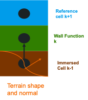
Terrain Model

An immersed boundary forcing method (IBFM) is used to represent the terrain. In this method, the effect of the terrain is modeled using a forcing term in the momentum and energy equation.

The forcing term in the momentum equation is given by:

\[F_i = - \beta C_d u_i | u_i |\]

Here \(\beta\) is the volume fraction of the cell covered by terrain, \(C_d\) is a drag term and \(u_i\) is the wind speed. Currently, the volume fraction is computed as a 0 or 1 using a simple nearest cell algorithm at each grid level. Future, updates will incorporate the partial terrain overlap using the EB capability in AMReX. The calculation of the drag coefficient term and the forcing term for the energy equation can be found in Muñoz‐Esparza, Domingo, et al. (JAMS 2020).

The original formulation is designed for low Reynolds number cases and does not include a method for applying a wall function. We propose the use of a forcing function to include the wall effects.

First, compute the friction velocity from location k+1:

\[u_*= |u_i[k+1]| \frac {\kappa}{\log [(z_{k+1}-z_k)/z0]}\]

The expected wind speed at cell k is computed as follows:

\[|u_n|= \frac{u_*}{\kappa} \log [0.5 (z_{k+1}-z_k)/z0]\]

The methodology can be extended to include stability functions in a straight forward manner. The forcing term is computed as

\[F_i= - \frac {|u[k]| \hat{c} - |u_n|\hat{l}} {\tau}\]

Here \(\hat{c}=(1,1,1)\) is the existing normal vector from the grid and \(\hat{l}=(ux,uy,0)/|u_n|\) is the value from the log law. The calculation of \(\hat{l}\) and \(u_*\) can be modified in the future align with the normal (following the orange arrow below).

Forest Model

The forest model provides an option to include the drag from forested regions to be included in the momentum equation. The drag force is calculated as follows:

\[F_i= - C_d L(x,y,z) U_i | U_i |\]

Here \(C_d\) is the coefficient of drag for the forested region and \(L(x,y,z)\) is the leaf area density (LAD) for the forested region. A three-dimensional model for the LAD is usually unavailable and is also cumbersome to use if there are thousands of trees. Two different models are available as an alternative:

\[L=\frac{LAI}{h}\]

\[L(z)=L_m \left(\frac{h - z_m}{h - z}\right)^n exp\left[n \left(1 -\frac{h - z_m}{h - z}\right )\right]\]

Here \(LAI\) is the leaf area index and is available from measurements, \(h\) is the height of the tree, \(z_m\) is the location of the maximum LAD, \(L_m\) is the maximum value of LAD at \(z_m\) and \(n\) is a model constant with values 6 (below \(z_m\)) and 0.5 (above \(z_m\)), respectively. \(L_m\) is computed by integrating the following equation:

\[LAI = \int_{0}^{h} L(z) dz\]

The simplified model with uniform LAD is recommended for forested regions with no knowledge of the individual trees. LAI values can be used from climate model look-up tables for different regions around the world if no local remote sensing data is available.

Turbine models

The modeling approaches for turbines, namely actuator disk model (ADM) and actuator line model (ALM), are presented in this section. Although AMR-Wind offers some stand-alone ADM implementations for turbines and ALM pathways for individual wings, the primary methods for turbine simulations rely on coupling with the modular, open-source, multifidelity wind-energy tool OpenFAST [Jonkman et al., 2018, NREL, 2023] for blade motion and turbine behavior while AMR-Wind calculates aerodynamic interactions.

Actuator disk model

The ADM is used to represent wind turbines as forces in the momentum equation [Aagaard Madsen, 1997, Calaf et al., 2010, Jimenez et al., 2007], spreading the induced forces over the swept area of the rotor (the disk). In this approach, the overall thrust force, \(F_t\), is generally calculated using the velocity averaged, \(\overline{u}\), over the rotor-swept area, \(\frac{\pi}{4} D^2\), and an empirically derived constant of thrust, \(C_t\), as shown by the formula

\[F_t = -\frac{1}{2}\rho \, C_t \overline{u}^2 \frac{\pi}{4} D^2.\]

The rotation of the turbine also introduces circulation in the flow via an azimuthal force, which has different representations depending on the model variant.

The forces are computed at discrete points on the disk surface using the actuator point \(i\), and these discrete forces are then spread over the turbine disk via a spreading function, \(\Gamma_i\), often a Gaussian [Martínez-Tossas et al., 2015]:

\[\Gamma_i(x_j) = \frac{1}{\epsilon^3\pi^{3/2}} \exp\bigg(-\frac{h_{i,j}^2}{\epsilon^2}\bigg), \label{eq:uniform_gauss}\]

where \(x_j\) is an arbitrary location in space, \(\epsilon\) is the characteristic width of the Gaussian kernel, and \(h_{i,j}\) is the distance between the actuator point \(i\) and the \(x_j\) position in space. A more general form of [eq:uniform_gauss] can be rewritten as a tensor product of contributions from each component of an orthogonal coordinate system:

\[\Gamma_i(x_j) = \eta (h_{i,1}) e_1 \otimes \psi (h_{i,2}) e_3 \otimes \vartheta (h_{i,3} ) e_3, \label{eq:nonuniform_gauss}\]

where \(\eta\), \(\psi\), and \(\vartheta\) represent different spreading kernels along the three principal coordinates (\(e_1\), \(e_2\), and \(e_3\)) of an orthogonal coordinate system.

AMR-Wind offers the traditional Gaussian along with a set of projections constructed from products of normalized linear basis functions, \(\xi\), similar to finite-elements, where the principal directions of the spreading functions align with the cylindrical coordinates of the disk. The geometry of the disk can be resolved with far fewer points because the linear basis functions form a partition of unity. The linear basis function can be expressed as

\[\xi_i(\tilde{x},\Delta h) = \frac{\max \left(0, 1-\frac{\vert \tilde{x}_i-\tilde{x} \vert}{\Delta h}\right)}{\Delta h}, \label{eq:linear-basis}\]

where \(\Delta h\) is the distance between the actuator points in the associated principal direction and \(\tilde{x}\) is the principal direction’s abscissa.

Employing the linear basis function, AMR-Wind offers a spreading function that is uniform in the \(\theta\) direction:

\[\Gamma_i(x_j) = \frac{\xi_r(r, \Delta r)}{2 \pi r_i} \: \frac{1}{\epsilon \sqrt{\pi}} \exp^{-\frac{\left(\tilde{z}_i-\tilde{z}_j\right)^2}{\epsilon^2}},\]

where \(r\) is the radial location along the disk and \(\tilde{z}\) is in the normal direction. Similarly, another option is available that discretizes in the \(\theta\) direction using arc length as the characteristic length scale:

\[\Gamma_i(x_j) = \xi_r(r, \Delta r) \: \xi_\theta(r\theta, r_i\Delta \theta) \: \frac{1}{\epsilon \sqrt{\pi}} \exp^{-\frac{\left(\tilde{z}_i-\tilde{z}_j\right)^2}{\epsilon^2}}.\]

Figure 1 illustrates the different ADM spreading-function approaches.

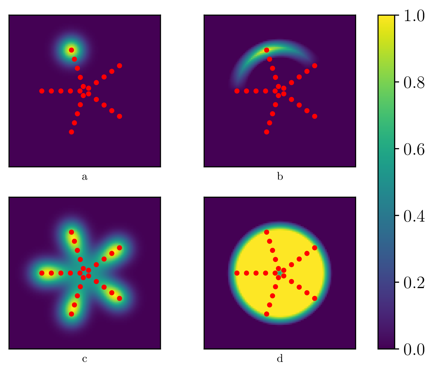
adm-disk-projections — 2 Illustration of actuator disk forcing using traditional point Gaussian functions (left) and using products of linear basis functions in the disk plane (right): (a) and (b) show the footprint of a single actuator point; (c) and (d) show the sum of all the points. The red dots indicate the location of the actuator points and the color bar shows the strength of a normalized force.

In conjunction with these spreading function options, AMR-Wind includes three implementations of the ADM, and in each case the wind speed is sampled at discrete points, spaced evenly across the disk. To accurately estimate the freestream velocity, sample points are also placed upstream of the turbine disk. At each sample point, the sampled wind velocity is obtained via linear interpolation. After the body forces are calculated according to the chosen method, they are applied to the flow at the discrete disk points. This means that the number of points for the wind speed sampling and the modeled body force can be independently configured for optimal sampling based on the chosen model and scenario.

The simplest of the ADM options in AMR-Wind is the uniform \(C_t\) model, which employs coefficients of thrust specified by the user at different wind speeds. To represent the loading on the blades, which directly translates to the force of the blades on the flow, the uniform \(C_t\) model applies the forcing term uniformly over each radial section of the disk. Further complexity is included in the Joukowsky disk model, described by [Sørensen et al., 2020] and updated in [Sørensen, 2023]. This model relies on an assumption of constant circulation over the disk with corrections for hub and tip effects, providing analytical expressions for axial and azimuthal force distributions. The Joukowsky disk approach has been validated for different wind turbines in diverse operating regimes and, as an analytical model, offers notable computational efficiency. Finally, AMR-Wind features an ADM approach coupled to OpenFAST [Cheung et al., 2023], whereby OpenFAST modules use the sampled wind speeds to calculate wind turbine dynamics, including the aerodynamics of the turbine blades. After calculating the resulting body forces, these are distributed back to the fluid domain within AMR-Wind by applying an isotropic smoothing kernel.

In some scenarios, the first two approaches may be more expedient, and they have the advantage of being fully contained within AMR-Wind. However, by coupling to OpenFAST, additional aspects of turbine behavior are included in the modeling framework, such as structural dynamics, and controllers can be easily incorporated to govern turbine behavior during the course of a simulation.

Actuator line model

The ALM is used to represent wings and individual wind turbine blades as body forces in the momentum equation [Martínez-Tossas et al., 2015, Sørensen and Shen, 2002, Troldborg et al., 2012], dividing the forces along a blade or wing into forces at actuator points along a line. In this approach, aerodynamic forces such as lift and drag are computed at each actuator point using a sampled velocity from the fluid solver and lookup tables for lift and drag coefficients, \(C_l\) and \(C_d\):

\[F_l = \frac{1}{2} \rho \, c \, w \, C_l (\alpha) \, U_{ rel}^2, ~~~~~~~~~~~~ F_d = \frac{1}{2} \rho \, c \, w \, C_d (\alpha) \, U_{ rel}^2,\]

where \(\alpha\) is the angle of attack, \(c\) is the local chord, \(w\) is the width of the blade element, and \(U_{rel}\) is the magnitude of the relative velocity [Martínez-Tossas et al., 2015, Sørensen et al., 2002]. The relative velocity vector, which contributes to \(\alpha\) and \(U_{rel}\), is calculated \(\boldsymbol{u}_{rel} = \boldsymbol{u}(\boldsymbol{x}_{i}) - \dot{\boldsymbol{x}}_{i}\), where \(\dot{\boldsymbol{x}}_i\) is the velocity of the actuator point \(i\), \(\boldsymbol{x}_i\) is the position of the actuator point \(i\), and \(\boldsymbol{u}(\boldsymbol{x}_i)\) is the sampled fluid velocity at that point. The lift force and drag force are then added in vector form and distributed around surrounding grid cells by using a finite Gaussian kernel:

\[\boldsymbol{S}_i(\boldsymbol{x}_j) = \frac{\boldsymbol{f}_i} {\epsilon_c \, \epsilon_t \, \epsilon_s \, \pi^{3/2}} \exp_{fin} \left( - \frac{x_c^2}{\epsilon_c} - \frac{x_t^2}{\epsilon_t} - \frac{x_s^2}{\epsilon_s} \right), \label{eq:lift-coord-spreading}\]

where \(\boldsymbol{f}_i=F_{l,i}\hat{e}_l + F_{d,i}\hat{e}_d\) is the aerodynamic force vector of an actuator point \(i\), \(x_c\), \(x_t\), and \(x_s\) are the distances from the center of the actuator point \(i\) to the point \(\boldsymbol{x}_j\) in the chord, thickness, and spanwise directions, and \(\epsilon_c\), \(\epsilon_t\), and \(\epsilon_s\) are the thickness of the Gaussian in the corresponding directions [Churchfield et al., 2017]. A finite Gaussian kernel is used to avoid calculating unreasonably small force values over the entire domain, and it is defined using

\[\begin{split}\exp_{fin}(-h^2) = \left\{\begin{matrix} \exp (-h^2) & \textrm{if } h < 4 \\ 0 & \textrm{otherwise} \end{matrix}\right. .\end{split}\]

The Godunov-based time discretization of AMR-Wind specifies that forcing terms, such as \(\boldsymbol{S}_i\) should be calculated at the half time step, \(n+1/2\). Calculating \(\boldsymbol{S}_i\) consists of two parts: the point-force vector \(\boldsymbol{f}_i\) and the Gaussian kernel centered at \((x_c,x_t,x_s)\). To get an accurate value of \(\boldsymbol{f}_i\), the velocity field must be sampled at the location of the actuator point, enabling the computation of the relative velocity \(U_{rel}\). Because the velocity field at \(n+1/2\) is not available when the point force needs to be calculated, we use the latest available information for this step; we sample the velocity field \(\boldsymbol{u}^n\) at the location of the actuator point at time step \(n\), which is \((x_c,x_t,x_s)^n\). Next, the Gaussian kernel translates the point force to a force field, centered at the actuator point. Because of the time discretization, we place the Gaussian kernel at the actuator location at time step \(n+1/2\), written as \((x_c,x_t,x_s)^{n+1/2}\). This location is straightforward to obtain through the turbine model interface: after sampling the velocity field and computing the point force, the turbine model advances to \(n+1\), providing the actuator point locations at \(n+1\). Actuator point locations at \(n+1/2\) are calculated through a simple arithmetic average:

\[(x_c,x_t,x_s)^{n+1/2} = \frac{1}{2}\left(x_c^n+x_c^{n+1},x_t^n+x_t^{n+1},x_s^n+x_s^{n+1} \right). \label{eq:alm_loc}\]

Because the accuracy of ALM relies on sampling the velocity at the location of the bound vortex [Martínez-Tossas et al., 2017], and this vortex is created from the inclusion of the source term \(\boldsymbol{S}_i\), the relationship between velocity sampling and force placement influences the accuracy of the method. Accuracy issues, such as dependence of the actuator force on the time step size and incorrect power estimation for the turbine, arise when [eq:alm_loc] is not used for the location of the actuator force, neglecting the time-staggered nature of AMR-Wind.

To simulate wind turbines using ALM, AMR-Wind relies on OpenFAST for the turbine representation. In this coupled framework, AMR-Wind supplies sampled velocities at actuator points to OpenFAST at the beginning of every time step, and OpenFAST returns updated actuator point forces and locations after progressing the turbine model forward in time. These forces and locations are incorporated into the AMR-Wind numerical algorithm through the actuator force implementation. By using OpenFAST, including aero-elastic deformations and changes in wind turbine operation is straightforward. These effects are computed by OpenFAST modules as the simulation evolves and are passed on to AMR-Wind as changes to the actuator point locations.

AMR-Wind offers a test bed for advanced actuator lines, providing variations to force distribution and point placement. The advanced ALM features include anisotropic Gaussian body forces to better represent wind turbine blades [Churchfield et al., 2012] and the filtered lifting line correction to obtain consistent results across different grid resolutions and \(\epsilon\) values [Dag and Sørensen, 2020, Martínez-Tossas and Meneveau, 2019, Martínez-Tossas et al., 2024].