Turbine simulation walkthrough
Now that we have run our precursor simulation and saved inflow boundary condition data, we can run a turbine simulation. Here is the input file:
  1#¨¨¨¨¨¨¨¨¨¨¨¨¨¨¨¨¨¨¨¨¨¨¨¨¨¨¨¨¨¨¨¨¨¨¨¨¨¨¨#
  2#            SIMULATION CONTROL         #
  3#.......................................#
  4time.stop_time                           = 7800.0       # Max (simulated) time to evolve [s]
  5time.max_step                            = -1           # Max number of time steps; -1 means termination set by timestamps
  6time.fixed_dt                            = 0.12         # Use this constant dt if > 0
  7time.cfl                                 = 0.95         # CFL factor
  8
  9time.plot_interval                       = 1250         # Steps between plot files
 10time.checkpoint_interval                 = 1250         # Steps between checkpoint files
 11ABL.bndry_file                           = ../precursor/bndry_file.native
 12ABL.bndry_io_mode                        = 1            # 0 = write, 1 = read
 13ABL.bndry_planes                         = xlo
 14ABL.bndry_output_start_time              = 7200.0
 15ABL.bndry_var_names                      = velocity temperature tke
 16
 17incflo.physics                           = ABL Actuator
 18io.restart_file                          = ../spinup/chk14400
 19io.outputs                               = "actuator_src_term"
 20turbulence.model                         = OneEqKsgsM84 # For neutral ABL, use "Smagorinsky"
 21TKE.source_terms                         = KsgsM84Src
 22incflo.gravity                           = 0.  0. -9.81 # Gravitational force (3D)
 23incflo.density                           = 1.225        # Reference density; make sure this agrees with OpenFAST values
 24transport.viscosity                      = 1.0e-5       # Dynamic viscosity [N-s/m^2]
 25transport.laminar_prandtl                = 0.7
 26transport.turbulent_prandtl              = 0.3333
 27transport.reference_temperature          = 290.0
 28
 29#¨¨¨¨¨¨¨¨¨¨¨¨¨¨¨¨¨¨¨¨¨¨¨¨¨¨¨¨¨¨¨¨¨¨¨¨¨¨¨#
 30#            GEOMETRY & BCs             #
 31#.......................................#
 32geometry.prob_lo                         = 0.       0.     0.   # Lo corner coordinates
 33geometry.prob_hi                         = 2560.  2560.  1280.  # Hi corner coordinates
 34amr.n_cell                               = 128 128 64           # Grid cells at coarsest AMRlevel
 35amr.max_level                            = 2                    # Max AMR level in hierarchy
 36geometry.is_periodic                     = 0   0   0            # Periodicity x y z (0/1)
 37
 38xlo.type                                 = mass_inflow
 39xlo.density                              = 1.225
 40xlo.temperature                          = 290.0
 41xlo.tke                                  = 0.0
 42xhi.type                                 = pressure_outflow
 43
 44ylo.type                                 = slip_wall
 45yhi.type                                 = slip_wall
 46
 47zlo.type                                 = wall_model
 48zhi.type                                 = slip_wall
 49zhi.temperature_type                     = fixed_gradient
 50zhi.temperature                          = 0.003
 51
 52#¨¨¨¨¨¨¨¨¨¨¨¨¨¨¨¨¨¨¨¨¨¨¨¨¨¨¨¨¨¨¨¨¨¨¨¨¨¨¨#
 53#               PHYSICS                 #
 54#.......................................#
 55ICNS.source_terms                        = BoussinesqBuoyancy CoriolisForcing BodyForce ABLMeanBoussinesq ActuatorForcing
 56##--------- Additions by calc_inflow_stats.py ---------#
 57ABL.wall_shear_stress_type = "local"
 58ABL.inflow_outflow_mode = true
 59ABL.wf_velocity = 7.612874161922772 0.05167978610261268
 60ABL.wf_vmag = 7.655337919472146
 61ABL.wf_theta = 291.0187046202964
 62# BodyForce.magnitude = 0.00034839850789284793 0.0009712494385077595 0.0
 63##-----------------------------------------------------#
 64BodyForce.uniform_timetable_file = "../precursor/abl_forces.txt"
 65incflo.velocity                          = 10.0 0.0 0.0
 66ABLForcing.abl_forcing_height            = 86.5
 67CoriolisForcing.latitude                 = 36.607322                 # Southern Great Plains
 68CoriolisForcing.north_vector             = 0.0 1.0 0.0
 69CoriolisForcing.east_vector              = 1.0 0.0 0.0
 70ABL.temperature_heights                  = 0.0 600.0 700.0 1700.0    # Make sure top height >= the domain height
 71ABL.temperature_values                   = 290.0 290.0 298.0 301.0
 72ABL.perturb_temperature                  = true
 73ABL.cutoff_height                        = 50.0
 74ABL.perturb_velocity                     = true
 75ABL.perturb_ref_height                   = 50.0
 76ABL.Uperiods                             = 4.0
 77ABL.Vperiods                             = 4.0
 78ABL.deltaU                               = 1.0
 79ABL.deltaV                               = 1.0
 80ABL.kappa                                = .40
 81ABL.surface_roughness_z0                 = 0.01  # [m]
 82ABL.surface_temp_flux                    = 0.05  # Surface temperature flux [K-m/s]
 83ABLMeanBoussinesq.read_temperature_profile = true
 84ABLMeanBoussinesq.temperature_profile_filename = avg_theta.dat
 85
 86#¨¨¨¨¨¨¨¨¨¨¨¨¨¨¨¨¨¨¨¨¨¨¨¨¨¨¨¨¨¨¨¨¨¨¨¨¨¨¨#
 87#          POST-Processing              #
 88#.......................................#
 89incflo.post_processing                   = sampling averaging
 90
 91# --- Sampling parameters ---
 92sampling.output_interval                = 100
 93sampling.fields                          = velocity temperature
 94
 95#---- sample defs ----
 96sampling.labels                          = xy-domain xz-domain
 97
 98sampling.xy-domain.type                  = PlaneSampler
 99sampling.xy-domain.num_points            = 256 256
100sampling.xy-domain.origin                = 0.0 0.0 91.0
101sampling.xy-domain.axis1                 = 2550.0 0.0 0.0
102sampling.xy-domain.axis2                 = 0.0 2550.0 0.0
103sampling.xy-domain.offset_vector         = 0.0 0.0 1.0
104sampling.xy-domain.offsets               = -63.45 0.0 63.45
105
106sampling.xz-domain.type                  = PlaneSampler
107sampling.xz-domain.num_points            = 256 128
108sampling.xz-domain.origin                = 0.0 1280.0 0.0
109sampling.xz-domain.axis1                 = 2550.0 0.0 0.0
110sampling.xz-domain.axis2                 = 0.0 0.0 1270.0
111
112#¨¨¨¨¨¨¨¨¨¨¨¨¨¨¨¨¨¨¨¨¨¨¨¨¨¨¨¨¨¨¨¨¨¨¨¨¨¨¨#
113#              AVERAGING                #
114#.......................................#
115averaging.type                           = TimeAveraging
116averaging.labels                         = means stress
117
118averaging.averaging_window               = 60.0
119averaging.averaging_start_time           = 7200.0
120
121averaging.means.fields                   = velocity
122averaging.means.averaging_type           = ReAveraging
123
124averaging.stress.fields                  = velocity
125averaging.stress.averaging_type          = ReynoldsStress
126
127#¨¨¨¨¨¨¨¨¨¨¨¨¨¨¨¨¨¨¨¨¨¨¨¨¨¨¨¨¨¨¨¨¨¨¨¨¨¨¨#
128#            MESH REFINEMENT            #
129#.......................................#
130tagging.labels                           = T0_level_0_zone T1_level_0_zone T2_level_0_zone T0_level_1_zone T1_level_1_zone T2_level_1_zone
131
132# 1st refinement level
133tagging.T0_level_0_zone.type             = GeometryRefinement
134tagging.T0_level_0_zone.shapes           = T0_level_0_zone
135tagging.T0_level_0_zone.level            = 0
136tagging.T0_level_0_zone.T0_level_0_zone.type = box
137tagging.T0_level_0_zone.T0_level_0_zone.origin = 520.0 1040.0 0.0  # -1D, -2D
138tagging.T0_level_0_zone.T0_level_0_zone.xaxis = 360.0 0.0 0.0
139tagging.T0_level_0_zone.T0_level_0_zone.yaxis = 0.0 480.0 0.0
140tagging.T0_level_0_zone.T0_level_0_zone.zaxis = 0.0 0.0 360.0
141
142tagging.T1_level_0_zone.type             = GeometryRefinement
143tagging.T1_level_0_zone.shapes           = T1_level_0_zone
144tagging.T1_level_0_zone.level            = 0
145tagging.T1_level_0_zone.T1_level_0_zone.type = box
146tagging.T1_level_0_zone.T1_level_0_zone.origin = 1160.0 1040.0 0.0  # -1D, -2D
147tagging.T1_level_0_zone.T1_level_0_zone.xaxis = 360.0 0.0 0.0
148tagging.T1_level_0_zone.T1_level_0_zone.yaxis = 0.0 480.0 0.0
149tagging.T1_level_0_zone.T1_level_0_zone.zaxis = 0.0 0.0 360.0
150
151tagging.T2_level_0_zone.type             = GeometryRefinement
152tagging.T2_level_0_zone.shapes           = T2_level_0_zone
153tagging.T2_level_0_zone.level            = 0
154tagging.T2_level_0_zone.T2_level_0_zone.type = box
155tagging.T2_level_0_zone.T2_level_0_zone.origin = 1800.0 1040.0 0.0  # -1D, -2D
156tagging.T2_level_0_zone.T2_level_0_zone.xaxis = 360.0 0.0 0.0
157tagging.T2_level_0_zone.T2_level_0_zone.yaxis = 0.0 480.0 0.0
158tagging.T2_level_0_zone.T2_level_0_zone.zaxis = 0.0 0.0 360.0
159
160# 2nd refinement level
161tagging.T0_level_1_zone.type             = GeometryRefinement
162tagging.T0_level_1_zone.shapes           = T0_level_1_zone
163tagging.T0_level_1_zone.level            = 1
164tagging.T0_level_1_zone.T0_level_1_zone.type = box
165tagging.T0_level_1_zone.T0_level_1_zone.origin = 580.0 1100.0 20.0  # -0.5D, -1.5D
166tagging.T0_level_1_zone.T0_level_1_zone.xaxis = 180.0 0.0 0.0
167tagging.T0_level_1_zone.T0_level_1_zone.yaxis = 0.0 360.0 0.0
168tagging.T0_level_1_zone.T0_level_1_zone.zaxis = 0.0 0.0 180.0
169
170tagging.T1_level_1_zone.type             = GeometryRefinement
171tagging.T1_level_1_zone.shapes           = T1_level_1_zone
172tagging.T1_level_1_zone.level            = 1
173tagging.T1_level_1_zone.T1_level_1_zone.type = box
174tagging.T1_level_1_zone.T1_level_1_zone.origin = 1220.0 1100.0 20.0  # -0.5D, -1.5D
175tagging.T1_level_1_zone.T1_level_1_zone.xaxis = 180.0 0.0 0.0
176tagging.T1_level_1_zone.T1_level_1_zone.yaxis = 0.0 360.0 0.0
177tagging.T1_level_1_zone.T1_level_1_zone.zaxis = 0.0 0.0 180.0
178
179tagging.T2_level_1_zone.type             = GeometryRefinement
180tagging.T2_level_1_zone.shapes           = T2_level_1_zone
181tagging.T2_level_1_zone.level            = 1
182tagging.T2_level_1_zone.T2_level_1_zone.type = box
183tagging.T2_level_1_zone.T2_level_1_zone.origin = 1860.0 1100.0 20.0  # -0.5D, -1.5D
184tagging.T2_level_1_zone.T2_level_1_zone.xaxis = 180.0 0.0 0.0
185tagging.T2_level_1_zone.T2_level_1_zone.yaxis = 0.0 360.0 0.0
186tagging.T2_level_1_zone.T2_level_1_zone.zaxis = 0.0 0.0 180.0
187
188#¨¨¨¨¨¨¨¨¨¨¨¨¨¨¨¨¨¨¨¨¨¨¨¨¨¨¨¨¨¨¨¨¨¨¨¨¨¨¨#
189#               TURBINES                #
190#.......................................#
191Actuator.labels                          = T0 T1 T2
192
193Actuator.TurbineFastDisk.density         = 1.225  # AirDens in OpenFAST models
194
195Actuator.T0.type                         = TurbineFastDisk
196Actuator.T0.openfast_input_file          = T0_OpenFAST/NREL-2p8-127.fst
197Actuator.T0.base_position                = 640.0 1280.0 0.0
198Actuator.T0.rotor_diameter               = 126.9
199Actuator.T0.hub_height                   = 86.5
200Actuator.T0.num_points_blade             = 64
201Actuator.T0.num_points_tower             = 12
202Actuator.T0.epsilon                      = 5.0 5.0 5.0
203Actuator.T0.epsilon_tower                = 5.0 5.0 5.0
204Actuator.T0.openfast_start_time          = 0.0
205Actuator.T0.openfast_stop_time           = 99999.0
206Actuator.T0.nacelle_drag_coeff           = 0.0
207Actuator.T0.nacelle_area                 = 0.0
208Actuator.T0.yaw                          = 0.0
209Actuator.T0.output_frequency             = 10
210
211Actuator.T1.type                         = TurbineFastDisk
212Actuator.T1.openfast_input_file          = T1_OpenFAST/NREL-2p8-127.fst
213Actuator.T1.base_position                = 1280.0 1280.0 0.0
214Actuator.T1.rotor_diameter               = 126.9
215Actuator.T1.hub_height                   = 86.5
216Actuator.T1.num_points_blade             = 64
217Actuator.T1.num_points_tower             = 12
218Actuator.T1.epsilon                      = 5.0 5.0 5.0
219Actuator.T1.epsilon_tower                = 5.0 5.0 5.0
220Actuator.T1.openfast_start_time          = 0.0
221Actuator.T1.openfast_stop_time           = 99999.0
222Actuator.T1.nacelle_drag_coeff           = 0.0
223Actuator.T1.nacelle_area                 = 0.0
224Actuator.T1.yaw                          = 0.0
225Actuator.T1.output_frequency             = 10
226
227Actuator.T2.type                         = TurbineFastDisk
228Actuator.T2.openfast_input_file          = T2_OpenFAST/NREL-2p8-127.fst
229Actuator.T2.base_position                = 1920.0 1280.0 0.0
230Actuator.T2.rotor_diameter               = 126.9
231Actuator.T2.hub_height                   = 86.5
232Actuator.T2.num_points_blade             = 64
233Actuator.T2.num_points_tower             = 12
234Actuator.T2.epsilon                      = 5.0 5.0 5.0
235Actuator.T2.epsilon_tower                = 5.0 5.0 5.0
236Actuator.T2.openfast_start_time          = 0.0
237Actuator.T2.openfast_stop_time           = 99999.0
238Actuator.T2.nacelle_drag_coeff           = 0.0
239Actuator.T2.nacelle_area                 = 0.0
240Actuator.T2.yaw                          = 0.0
241Actuator.T2.output_frequency             = 10
This file looks like the precursor input file, except for the following changes:
We are now reading in boundary condition data, not writing it out. Similarly, the x- and y- boundaries are no longer periodic, requiring us to specify some extra characteristics about the inflow.
We added the line
io.outputs="actuator_src_term"to output relevant information about the location of the turbines for plotting purposesincflo.physicsnow includesActuatorso that turbine-related calculations can take place.Similarly, we remove
ABLForcingfromICNS.source_terms, and we replace it with three new forces:BodyForce ABLMeanBoussinesq ActuatorForcing. We then provide extra information about these forces. More on how to calculate these values down below.We also add details under
ABLto inform the wall function.We add information about the turbines and surrounding mesh refinements into the input file. Because of the finer mesh, the small dt is required for this simulation.
time.fixed_dtis changed from 0.125 to 0.12. Although 0.125 is sufficient for the finer mesh in this simulation, there is an additional constraint of compatibility with the OpenFAST turbine model. The AMR-Wind time step size must be an integer multiple of the recommended time step size of the turbine model (written asDTin the.fstOpenFAST input). For this turbine model, the recommended DT is 0.01, requiring a change to the AMR-Wind dt. Due to this change in the time step size, we have also adjusted the plotting, checkpoint, and sampling intervals.
Further details about these source terms and wall function (wf) specifications
Now that this simulation is not periodic and will feature turbine wakes, the previous approach to forcing the velocity field (ABLForcing) is not viable. In addition to the inflow information from the precursor simulation, we also want to mimic the forcing terms. This is the purpose of BodyForce.
ABLMeanBoussinesq modifies the BoussinesqBuoyancy term to make it reference a profile of average temperature values instead of a single reference temperature. Instead of modifying the physics, this term is intended to modify the pressure distribution to make it more compatible with the outflow condition.
ActuatorForcing indicates to the momentum equation that terms from the actuator turbine model should be included. Both the Actuator physics instance and the source_term specification need to be present for the simulation to run as intended.
Similar to how ABLForcing is not a viable option in an inflow-outflow simulation with turbines, wall function implementations that rely on planar averages are not viable either. Instead, time averages of planar-averaged precursor data from is passed to the inflow-outflow simulation to inform that wall model.
When running an inflow-outflow simulation, information must be provided for the new source terms and the wall function. These
values are intended to be statistical data calculated from the precursor simulation. During the precursor, ABL Stats
output planar-averaged data at discrete times. To average this data in time and obtain values for the input arguments,
applying a script is the most direct approach. For this step, run the calc_inflowoutflow_stats.py script, provided in
the tools directory of the AMR-Wind repo, as follows:
python <path to amr-wind repo>/tools/calc_inflowoutflow_stats.py -sf <path to precursor directory>/post_processing/abl_statistics14400.nc -ts 7200 -te 7800
The -ts and -te arguments communicate the start time and end time for the time averaging, respectively. Running the
script provides two important things:
Complete input lines to be copy-pasted into the turbine input file, which feature time-averaged information
An
avg_theta.datfile with an average temperature profile forABLMeanBoussinesq. It is critical that this file is available where the job will run; otherwise, AMR-Wind will fail by not being able to find the file.
Although the script provides a value for the BodyForce.magnitude, this has been commented out after being pasted into the
input file. This is because we prefer to use a timetable for the body force, which was output by the precursor simulation.
If the forcing_timetable_output_file argument is not used in a precursor simulation setup, this timetable file will not be available.
In that case, using a constant, uniform body force vector is the standard approach, and this script provides the
time-averaged value from the precursor to populate BodyForce.magnitude.
Because we are simulating turbines, OpenFAST files need to be included for each of the turbines. In this walkthrough, we use 2.8 MW turbines from NREL’s open source turbine repository, and the specific turbine model is here.
Instead of cloning the entire repository of OpenFAST turbine models, we can clone only what is needed to run the full turbine simulation and then copy it to the run directory.
First, clone the repository as empty and enter its directory.
git clone -n --depth=1 --filter=tree:0 https://github.com/NREL/openfast-turbine-models.git && cd openfast-turbine-models
Then, check out only the path that we need.
git sparse-checkout set --no-cone IEA-scaled/NREL-2.8-127/20_monolithic_opt2/OpenFAST && git checkout
cd IEA-scaled/NREL-2.8-127/20_monolithic_opt2/OpenFAST/
Note that, when simulating OpenFAST turbines through AMR-Wind instead of directly through OpenFAST, it is important to make the following changes to the OpenFAST files:
NREL-2p8-127_AeroDyn15.dat: Make sureWakeModis0NREL-2p8-127_ElastoDyn.dat: Set the initial RPMRotSpeedand initial yaw angleNacYawto reasonable values (in this walkthrough we use13.5RPM and0degrees, respectively)NREL-2p8-127.fst: SetCompInflowto be2andOutFileFmtto be1NREL-2p8-127_ServoDyn.dat: Make sureDLL_FileNamepoints to alibdiscon.so(on Linux) orlibdiscon.dylib(on Mac) file from ROSCO. If you compiled using exawind-manager, see the section of the documentation that discusses how to determine the correct path to this ROSCO library file.
After performing these changes, copy the OpenFAST model to the run directory using the names in the AMR-Wind input file.
cd ..
cp -r OpenFAST/ <path to turbine run directory>/T0_OpenFAST
cp -r OpenFAST/ <path to turbine run directory>/T1_OpenFAST
cp -r OpenFAST/ <path to turbine run directory>/T2_OpenFAST
When all of these steps are complete, the job directory for running the turbine simulation includes
avg_theta.dat T0_OpenFAST/ T1_OpenFAST/ T2_OpenFAST/ turbines.inp
and the turbine inflow-outflow simulation is ready to be submitted using
amr_wind turbines.inp
which should follow after an srun or mpiexec or a similar command to take advantage of parallelization.
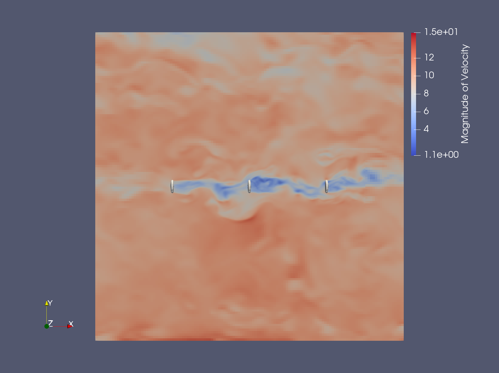
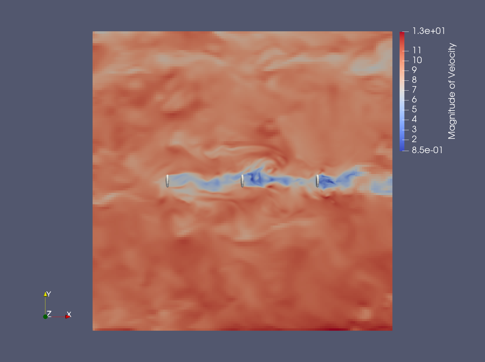
Below we show the magnitude of the velocity at t=7350s (top) and at the final time
(bottom) of the simulation. In both images, the three turbines are displayed as 3D
contours of the actuator_src_termx field. Note the turbine-induced wakes
and their impact on the incoming flow for the downstream turbines.