Postprocessing NREL5MW AMR-Wind results
Contents
The following document describes the post-processing procedures for the AMR-Wind turbine simulation.
Note: In many of the python scripts and Jupyter notebooks provided, the path to the AMR-Wind front end library must be provided. If necessary, download the library and edit the lines in the python code which define amrwindfedirs to include any locations of that library.
# Add any possible locations of amr-wind-frontend here
amrwindfedirs = ['/projects/wind_uq/lcheung/amrwind-frontend/',
                 '/ccs/proj/cfd162/lcheung/amrwind-frontend/']
import sys, os, shutil, io
for x in amrwindfedirs: sys.path.insert(1, x)
OpenFAST turbine results
Jupyter notebook: OpenFAST_v40_Results.ipynb
python script: OpenFAST_v40_Results.py
These scripts extract out specific performance quantities from the OpenFAST output files and creates a time history of quantities to compare, as well as averaging them over a specific time period. To use the scripts and notebooks above, change the RUNDIR variable in the replacedict definition:
replacedict={'RUNDIR':'/nscratch/gyalla/HFM/exawind-benchmarks/amr-wind/NREL5MW_ALM_BD/runs/',
             'RESULTSDIR':'../results/OpenFAST_v402_out',
             'RESULTSOLDDIR':'../results/OpenFAST_out'
            }
Inside the yamlstring variable, also double-check the trange variable to make sure the averaging time is correct:
trange: &trange [300, 900] # Note: add 15,000 sec to get AMR-Wind time
Then execute and run the notebook/script and it will extract the results.
$ python OpenFAST_v40_Results.py
The outputs of the script are contained in two CSV files:
NREL5MW.csv: A time history of turbine parameters such as blade pitch, rotor speed, rotor thrust, rotor torque, and generator power.
NREL5MW_mean.csv: The time average of the turbine properties over the time period defined by
trange.
Plots of the quantities from NREL5MW.csv are also generated in the images directory, look for the OpenFAST_T0_*.png files.
OpenFAST blade loading profiles
Jupyter notebook: OpenFAST_SectionalLoading.ipynb
python script: OpenFAST_SectionalLoading.py
Similar to the scripts which extract the time-history of the turbine quantities above, the notebook and python script above extract the blade loading profiles from the OpenFAST output file. These include the radial distributions of angle of attack, lift/drag coefficients, and streamwise/tangential blade forces.
In the notebook and python script, edit the locations of the files in these variables
rundir = '/gpfs/lcheung/HFM/exawind-benchmarks/NREL5MW_ALM_BD_OFv402_ROSCO/'
bladefile = rundir+'/T0_NREL5MW_v402_ROSCO/openfast/5MW_Baseline/NRELOffshrBsline5MW_AeroDyn_blade.dat'
and define the list of variables to extract here:
suffixkeys = ['Alpha', 'Phi', 'Cl','Cd', 'Fx','Fy']
The time range to average the data is defined in trange:
trange: &trange [300, 900] # Note: add 15,000 sec to get AMR-Wind time
The raw output will be stored in the file NREL5MW_SECLOADS_mean_rpts.csv. Plots of the blade loading are also generated in the images directory, in the files:
OpenFAST_T0_AOA.png
OpenFAST_T0_ClCd.png
OpenFAST_T0_FxFy.png
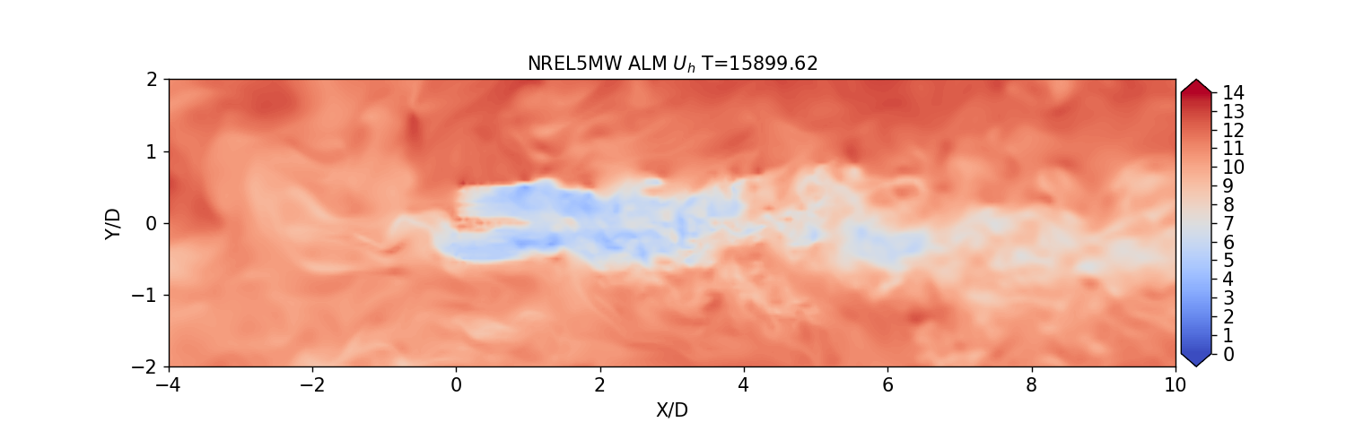
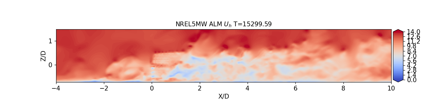
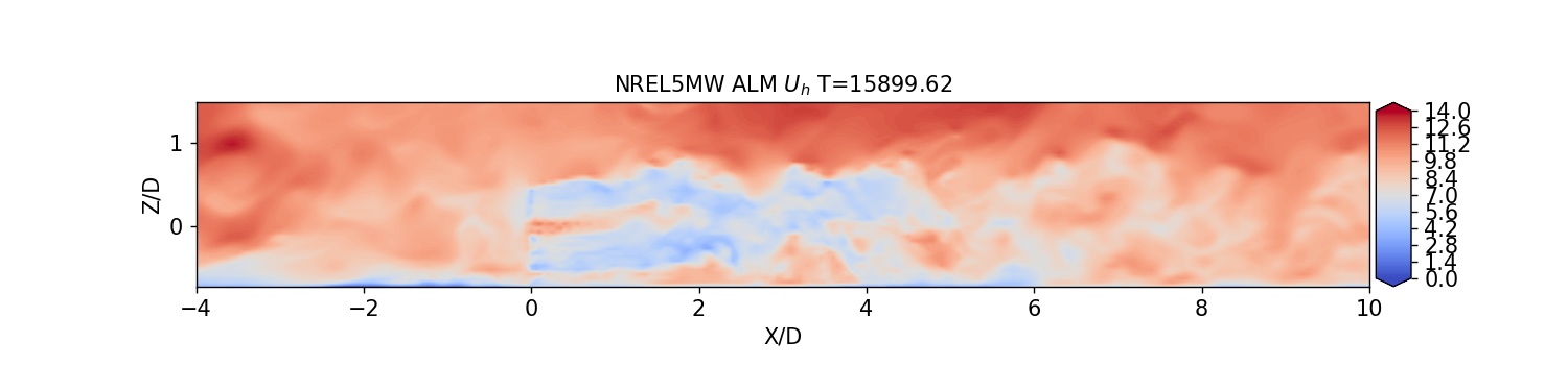
Contour plots
Jupyter notebook: InstantaneousAvgPlanes.ipynb
python script: InstantaneousAvgPlanes.py
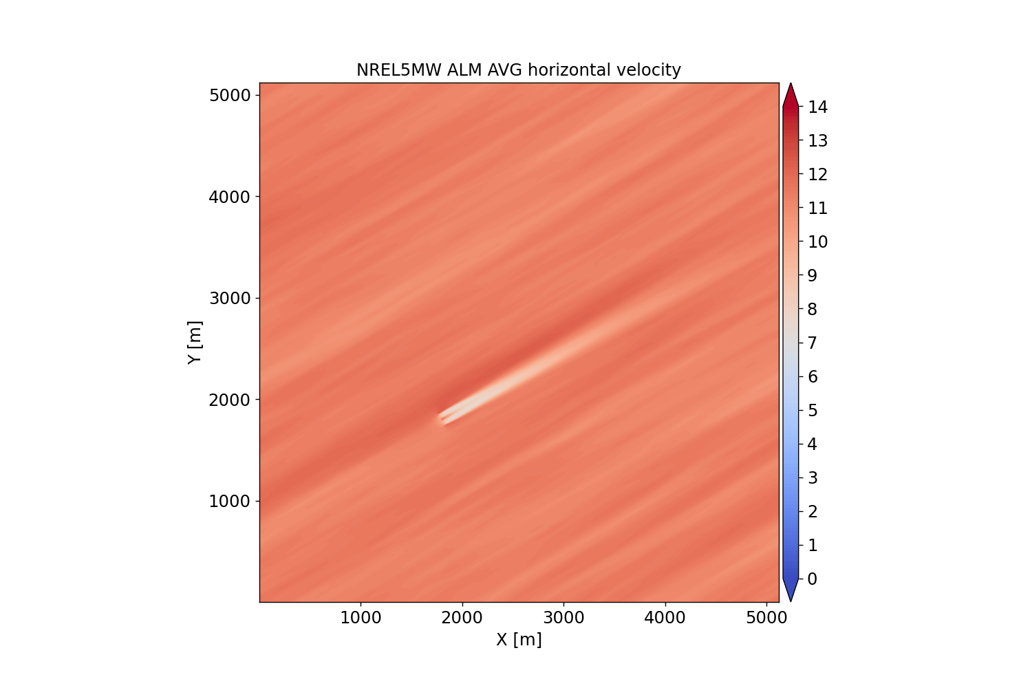
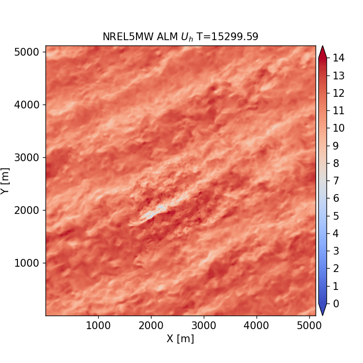
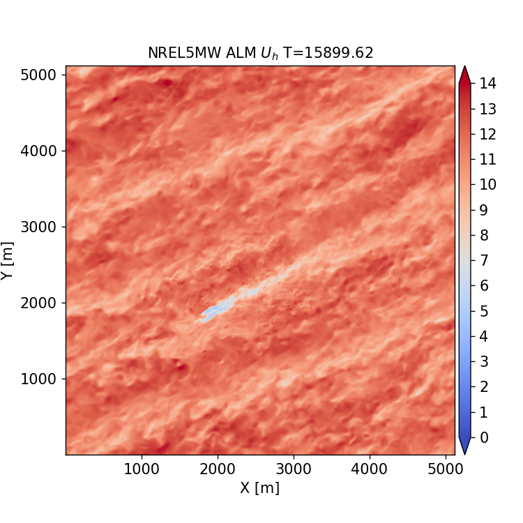
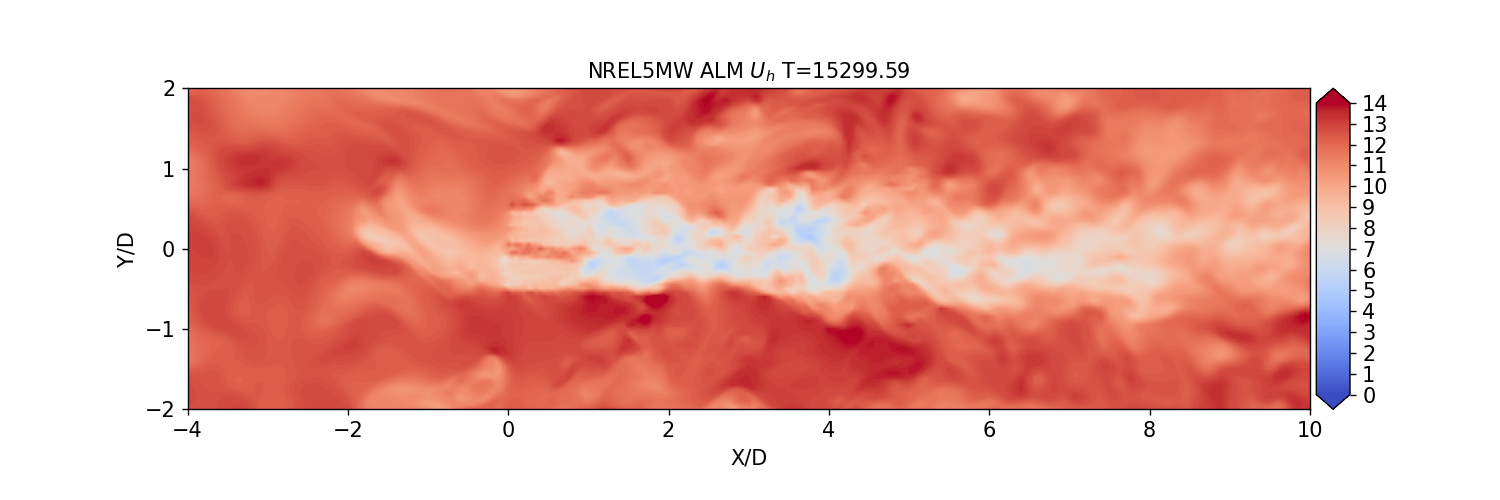
Images of the domain and the flow-field around the turbine are generated using the Jupyter notebook and python script above. The notebook and script will extract hub-height and streamwise slices from the sampling planes that were generated from AMR-Wind. They will also perform a time-average of the hub-height plane through the entire domain for a quick visualization.
To use the postprocessing script and notebook, edit the RUNDIR to reflect the location of the AMR-Wind run.
replacedict={'RUNDIR':'/gpfs/lcheung/HFM/exawind-benchmarks/NREL5MW_ALM_BD_OFv402_ROSCO/',
            }
Also, if necessary, change the time period specified in trange. Currently it is set to do a 10-min average of the simulation after the initial transient period.
trange: &trange [15300, 15900]
After running the notebook, it should generate the following images from the domain:
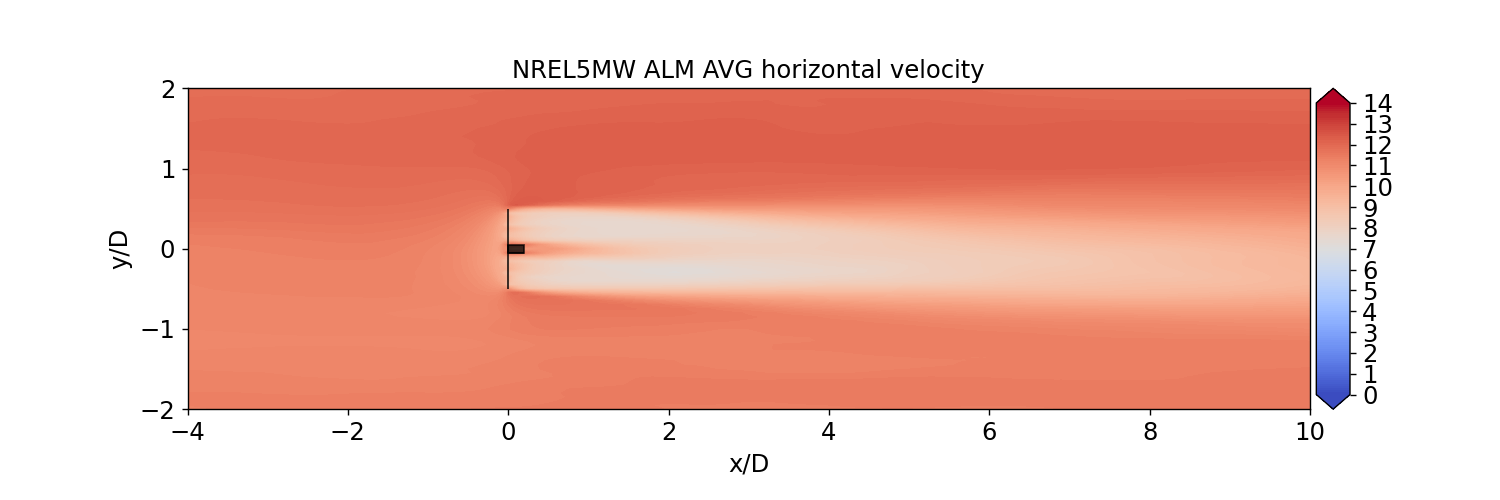
Averaged wake profiles
Jupyter notebook: AVGPlanes.ipynb
python script: AVGPlanes.py
These postprocesssing notebook and python script will extract hub-height and streamwise wake profiles from the sampling planes generated by AMR-Wind.
The time range to average the profiles is defined by the trange variable. Currently it is set to compute a 10 minute average after an initial 5 minute transient period:
trange: &trange [15300, 15900]
The locations of the hub-height wake profiles are defined by the interpXY user-defined function. Currently it creates profiles at x/D = 1,2,3, … 9 downstream, and from -2 <= y/D <= 2 laterally with 1 meter resolution. The results are stored in the results/HHProfiles_300_900 subdirectory.
def interpXY(xD):
    """
    Interpolate on the XY hub-height plane plane
    """
    D  = 126.0
    x0 = D*4.0
    y0 = D*2.0
    z0 = 90.0
    x = D*xD
    ptlist = [[x+x0, y+y0] for y in np.linspace(-D*2, D*2, int(D*4+1))]
    return ptlist

for x in [1,2,3,4,5,6,7,8,9,10]:
    setattr(ppeng, 'interpXY'+repr(x), partial(interpXY, x))
The locations of the streamwise profiles are defined by the interpXZ user-defined function. Currently it creates profiles at x/D = 1,2,3, … 10 downstream, and from 0 < z/D <= 2 with 1 meter resolution. The results are stored in the results/XZProfiles_300_900 subdirectory.
def interpXZ(xD):
    """
    Interpolate on the XZ streamwise plane
    """
    D  = 126.0
    x0 = D*4.0
    y0 = 0
    x = D*xD
    ptlist = [[x+x0, y+y0] for y in np.linspace(1, D*2, int(D*2))]
    return ptlist

for x in [1,2,3,4,5,6,7,8,9,10]:
    setattr(ppeng, 'interpXZ'+repr(x), partial(interpXZ, x))
Averaged contour plots for both the hub-height and the streamwise cases are also created and saved:
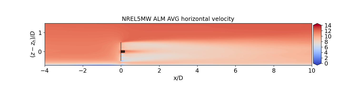