2. 2D Unsteady Uniform Property: Convecting Decaying Taylor Vortex

Verification of first-order and second-order temporal accuracy for the CVFEM and EBVC formulation in Nalu-Wind is performed using the method of manufactured solution (MMS) technique. For the unsteady isothermal, uniform laminar physics set, the exact solution of the convecting, decaying Taylor vortex is used.

(2.38)$$u=u_o-cos(\pi (x-u_{o}t))sin(\pi (y-v_{o}t))e^{-2.0\omega t}$$

(2.39)$$v=v_o+sin(\pi (x-u_{o}t))cos(\pi (y-v_{o}t))e^{-2.0\omega t}$$

(2.40)$$p=-\frac{p_o}{4}(cos(2\pi (x-u_{o}t))+cos(2\pi (y-v_{o}t)))e^{-4\omega t}$$

In this study, the constants $u_o$, $v_o$, and $p_o$ are all assigned values of $1.0$, and the viscosity $\mu$ is set to a constant value of $0.001$. The value of $\omega$ is ${\pi }^2\mu$. This particular viscosity value results in a maximum cell reynolds number of twenty.

2.1. Temporal Order Of Accuracy Results

The temporal order of accuracy for the first order backward Euler and second order BDF2 are outlined in Figure 2.2 and Figure 2.3. Each of these simulations used a hybrid factor of zero to ensure pure second order central usage. A fixed Courant number of two was used for each of the three meshes (100x100, 200x200 and 400x400). The simulation was run out to 0.2 seconds and $L_2$ error norms were computed. The standard fourth order pressure stabilization scheme with time step scaling is used. This scheme is also known as the standard incremental pressure, approximate pressure projection scheme.

Two other pressure projection schemes have been evaluated in this study. Each represent a simplification of the standard pressure projection scheme. Figure 2.4 outlines three projection schemes: the first is when the projected nodal gradient appearing in the fourth-order pressure stabilization is lagged while the second is the classic pressure-free pressure approximate projection scheme with second order pressure stabilization. The third is the baseline fourth-order incremental pressure projection scheme. The error plots demonstrate that lagging the projected nodal gradient for pressure retains second order accuracy. However, as expected the pressure free pressure projection scheme is confirmed to be first order accurate given the first order splitting error noted in this fully implicit momentum solve.

The Steady Taylor Vortex will be used to verify the spatial accuracy for the full set of advection operators supported in Nalu-Wind.

2.2 Error norms as a function of timestep size for the $u$ and $v$ component of velocity using fourth order pressure stabilization with timestep scaling, backward Euler

2.3 Error norms as a function of timestep size for the $u$ and $v$ component of velocity using fourth order pressure stabilization with timestep scaling, BDF2

2.4 Error norms as a function of timestep size for the $u$ and $v$ component of velocity using the lagged projected nodal pressure gradient and pressure-free pressure projection scheme; all with with timestep scaling, BDF2

3. Higher Order 2D Steady Uniform Property: Taylor Vortex

A higher order unstructured CVFEM method has been developed by Domino [Dom14]. A 2D structured mesh study demonstrating second order time and third order in space scheme has been demonstrated. The below work has emphasis on unstructured meshes.

3.1. Source Term Quadrature

Higher order accuracy is only demonstrated on solutions with source terms when a fully integrated approach is used. Lumping the source term evaluation is a second order error and is fully noted in the MMS study (not shown).

3.2. Projected nodal gradients

Results show that one must use design order projected nodal gradients. Figure 3.4 demonstrates a code verification result for a steady thermal manufactured solution comparing lumped and consistent mass matrix approaches for the projected nodal gradient on a quadratic tquad mesh. In the lumped approach, a simple explicit algorithm is processed while for the consistent approach, a simple mass matrix inversion equation must be solved. The lumped approach is first order while the consistent approach retains the expected second order as the projected nodal gradient is expected to be order $P$. Both Dirichlet and periodic domains display the same order of convergence.

3.4 Error norms as a function of mesh size for a CMM and LMM projected nodal gradient on a quadratic tquad mesh.

3.3. Momentum and Pressure

The steady taylor vortex exact solution was run on a quadratic tquad mesh. Figure 3.5 demonstrates the order of accuracy for projected nodal gradients (pressure) and the velocity field (x-component). Second order accuracy for the projected nodal gradient (pressure) and third order for the velocity field is realized when the consistent mass matrix approach is used for the projected nodal pressure gradient. Note that this term is used in the pressure stabilization approach. However, order of convergence for the projected nodal pressure gradient and velocity field is compromised when the lumped mass matrix approach is used for the pressure stabilization term. Note that both approaches use the fully integrated pressure gradient term in the momentum equation (i.e., $\int p{n}_{i}dS$). Therefore, the reduced order of integration for the projected nodal pressure gradient has consequence on the velocity field order of convergence.

Again, dirichlet (inflow) and periodic domains display the same order of convergence.

3.5 Error norms as a function of mesh size for the Steady Taylor Vortex momentum and pressure gradient field.

4. 3D Steady Non-isothermal with Buoyancy

Building from the basic functional form of the Taylor Vortex, a non-isothermal solution (momentum, pressure and static enthalpy) is manufactured as follows:

(4.11)$$\begin{array}{rl}u& =-u_{o}cos(a\pi x)sin(a\pi y)sin(a\pi z)\\ v& =+v_{o}sin(a\pi x)cos(a\pi y)sin(a\pi z)\\ w& =-w_{o}sin(a\pi x)sin(a\pi y)cos(a\pi z)\\ p& =-\frac{p_o}{4}(cos(2a\pi x)+cos(2a\pi y)+cos(2a\pi z))\\ h& =+h_{o}cos(a_h\pi x)cos(a_h\pi y)cos(a_h\pi z)\end{array}$$

The equation of state is simply the ideal gas law,

(4.12)$$\rho =\frac{P^{ref}M}{RT}$$

The simulation is run on a three-dimensional domain ranging from -0.05:+0.05 with constants $a,a_h,M,R,C_p,P^{ref},T_{ref},Pr,\mu$ equal to (20, 10, 30, 10, 0.01, 100, 300, 0.8, 0.00125), respectively.

At reference conditions, the density is unity. The effects of buoyancy are also provided by an arbitrary gravity vector of magnitude of approximately ten, $g_i=(-5,6,7{)}^T$. On this domain, the enthalpy ranges from zero to unity. Given the reference values, the temperature field ranges from 300K to 400K which is designed to mimic a current LES non-isothermal validation suite.

Edge- and element-based discretization (P=1) demonstrate second order convergence in the $L_2$ norm for u, v, w and temperature. This test is captured within the variableDensityMMS regression test suite.

5. 3D Steady Non-uniform with Buoyancy

Building from the basic functional form of the Taylor Vortex, a non-uniform solution (momentum, pressure and mixture fraction) is manufactured as follows:

(5.2)$$\begin{array}{rl}u& =-u_{o}cos(a\pi x)sin(a\pi y)sin(a\pi z)\\ v& =+v_{o}sin(a\pi x)cos(a\pi y)sin(a\pi z)\\ w& =-w_{o}sin(a\pi x)sin(a\pi y)cos(a\pi z)\\ p& =-\frac{p_o}{4}(cos(2a\pi x)+cos(2a\pi y)+cos(2a\pi z))\\ z& =+z_{o}cos(a_z\pi x)cos(a_z\pi y)cos(a_z\pi z)\end{array}$$

The equation of state is simply the standard inverse mixture fraction property expression for density,

(5.3)$$\rho =\frac{1}{\frac{z}{rh{o}^P}+\frac{1-z}{rh{o}^S}}$$

The simulation is run on a three-dimensional domain ranging from -0.05:+0.05 with constants $a,a_z,{\rho }^p,{\rho }^s,Sc,\mu$ equal to (20, 10, 0.1, 1.0, 0.8, 0.001), respectively.

At reference conditions, the density is that of the primary condition (0.1). The effects of buoyancy are also provided by an arbitrary gravity vector of magnitude of approximately ten, $g_i=(-5,6,7{)}^T$. On this domain, the mixture fraction ranges from zero to unity. This test case is designed to support the helium plume DNS study with primary and secondary density values of helium and air, respectively.

Edge- and element-based discretization (P=1) demonstrate second order convergence in the $L_2$ norm for u, v, w and mixture fraction. This test is captured within the variableDensityMMS regression test suite.

6. 2D Steady Laplace Operator

The evaluation of the low-Mach Laplace (or diffusion operator) is of great interest to the core supported application space. Although the application space for Nalu-Wind is characterized by a highly turbulent flow, the usage of an approximate pressure projection scheme always makes the chosen Laplace form important. Although the element-based scheme is expected to be accurate, it can be problematic on high aspect ratio meshes as element-based schemes are not gauranteed to be monotonic for aspect ratios as low as $\sqrt{2}$ for FEM-based schemes and $\sqrt{3}$ for CVEM-based approaches (both when using standard Gauss point locations). Conversely, while the edge-based operator is accurate on high aspect ratio meshes, it suffers on skewed meshes due to both quadrature error and the inclusion of a non orthogonal correction (NOC).

In order to assess the accuracy of the Laplace operator, a the two-dimensional MMS temperature solution is used. The functional temperature field takes on the following form:

(6.17)$$T=\frac{\lambda }{4}(cos(2a\pi x)+cos(2a\pi y)).$$

The above manufactured solution is run on three meshes of domain size of 1x1. The domain was first meshed as a triangular mesh and then converted to a tquad4 mesh. Therefore, non orthogonal correction (NOC) effects are expected for the edge-based scheme. In this study, both $\lambda$ and $a$ are unity. Either periodic or Dirichlet conditions are used for boundary conditions.

A brief overview of the diffusion operator tested is now provided. For more details, consult the theory manual. The general diffusion kernel is as follows:

(6.18)$$-\int \mathrm{\Gamma }\frac{\partial \varphi }{\partial x_j}{A}_j.$$

The choice of the gradient operator at the integration point is a functin of the underlying method. For CVFEM, the gradient operator is provided by the standard shape function derivatives,

(6.19)$$\frac{\partial {\varphi }_{ip}}{\partial x_j}=\sum \frac{\partial N_{j,k}^{ip}}{\partial x_j}{\varphi }_k.$$

For the edge-based scheme, a blending of an orthogonal gradient along the edge and a NOC is employed,

(6.20)$$\frac{\partial {\varphi }_{ip}}{\partial x_j}=\overline{G_j\varphi }+[({\varphi }_R-{\varphi }_L)-\overline{G_l\varphi }d{x}_l]\frac{A_j}{A_{k}d{x}_k}.$$

In the above equation, $G_j\varphi$ is a projected nodal gradient. The general equation for this quantity is

(6.21)$$\int w_I{G}_j\varphi dV=\int w_i\frac{\partial \varphi }{\partial x_j}dV.$$

Possible forms of this include either lumped or consistent mass (the later requires a global equation solve) with either the full CVFEM stencil or the edge-based (reduced) stencil. The above equation can even be applied within the element itself for a simple, local integration step that provides a piecewise constant gradient over the element.

The simulation study is run with the following diffusion operators: 1) the standard CVFEM operator, 2) the edge-based operator with CVFEM projected nodal gradients (NOC), 3) the edge-based operator with edge-based projected nodal gradients (NOC), 4) the edge-based operator without NOC correction, 5) the CVFEM operator with shifted integration points to the edge, and, lastly, 6) a mixed edge/element scheme in which the orthogonal diffuion operator is edge-based while the NOC terms are based on the elemental CVFEM gradient (either evaluated at the given integration point or integrated over the element for a piecewise constant form).

The last operator is interesting in that it represents a candidate operator for the CVFEM pressure Poisson system when high aspect ratio meshes are used. Figure 6.1 outlines the convergence of the five above operators; shown are all of the standard norms ($\mathrm{\infty }$, $1$ and $2$) for the R0, R1 and R2 mesh refinements. The results in the left side of the figure indicate that the edge-based scheme with NOC retains second-order convergence for all norms when the more accurate CVFEM projected nodal gradient is used (lumped only tested given its good results). Convergence is degraded with the edge-based scheme when NOC terms are either neglected or use the reduced edge-based projected nodal gradient. The CVFEM-based methods are second order accurate in the $L_1$ and $L_2$ norms, however, questionable results are noted in the $L_{\mathrm{\infty }}$ norm for all methods that include any shape function derivative for local or elemental piecwise constant gradient operators. Shifting the Gauss points from the standard subcontrol surface to the edges of the element (while still using shape function derivatives) is only problematic in the $L_{\mathrm{\infty }}$ norm (just as the standard CVFEM approach). The use of the mixed-approach with a piecewise constant gradient over the element demonstrates the same behavior as when using the integration point CVFEM gradient operator. Figure 6.2 outlines two more refinement meshes for the CVFEM operator (R3 and R4). Results indicate that the $L_{\mathrm{\infty }}$ norm is approaching second order accuracy.

6.1 Error norms for tquad4 refinement study. R0, R1, and R2 refinement.

6.2 Error norms for tquad4 refinement study. R0, R1, R2, R3, R4, and R4 refinementError for CVFEM.

An inspection of the magnitude of error between the exact and computed temperature for the R3 mesh is shown in Figure 6.3. Results show that the CVFEM error is highest at the corner mesh nodes that form a reduced stencil. The edge-based scheme shows increased error at the higher aspect ratio dual mesh.

6.3 Magnitude of the $L_{\mathrm{\infty }}$ temperature norm comparing the edge-based CVFEM (NOC) and standard CVFEM operators on the R3 mesh.

7. 3D Steady Laplace Operator with Nonconformal Interface

A three dimensional element-based verification study is provided to evaluate the DG-based CVFEM approach.

(7.16)$$T=\frac{\lambda }{4}(cos(2a\pi x)+cos(2a\pi y)+cos(2a\pi z)).$$

Figure 7.1 represents the MMS field for temperature. The simulation study includes uniform refinement of a first- and second-order CVFEM basis. Both temperature field and projected nodal gradient norms are of interest.

7.1 MMS temperature field for nonconformal algorithm.

Figure 7.2 outlines the linear and quadratic basis. For P1, the CVFEM temperature field predicts between second and first order while for P2, third order is recovered. When using a consistent mass matrix for the projected nodal gradient, second order is noted, see Figure 7.3.

7.2 MMS order of accuracy for nonconformal algorithm. Temperature norms for P1 and P2 elements.

7.3 MMS order of accuracy for nonconformal algorithm. Projected nodal gradient norms for P1 and P2 elements.

7.1 Patch test

dof	$L_{\mathrm{\infty }}$	L1	L2
temperature	3.33067e-16	2.30077e-17	4.68103e-17
dTdx	4.13225e-13	9.06848e-15	1.98249e-14
dTdy	4.15668e-13	1.11256e-14	2.15065e-14
dTdz	4.31211e-13	9.60785e-15	1.97517e-14

Given the order of accuracy results for the P1 implementation, a linear patch test was run. The temperature solution was simply, $T(x,y,z)=x+y+z$; all analytical temperature gradients are unity. Table 7.1 demonstrates the successful patch test results for a P1 CVFEM implementation.

8. Precursor-based Simulations

In the field of turbulent flow modeling and simulation, often times simulations may require sophisticated boundary conditions that can only be obtained from previously run high-fidelity simulations. For example, consider a typical turbulent jet simulation in which the experimental inlet condition was preceeded by a turbulent pipe entrance region. Furthermore, in most cases the ability to adequately predict the developing jet flow regime may be highly sensitive to proper inlet conditions. Figure 8.1 and Figure 8.2 outline a process in which a high fidelity large-eddy simulation of a periodic pipe was used to determine a representative inlet condition for a turbulent round jet. Specifically, a precursor pipe flow simulation is run with velocity provided to an output file. This output file serves as the inlet velocity profile for the subsequent simulation.

8.1 Precursor periodic pipe flow large-eddy simulation that will serve as the inlet boundary condition for a subsequent turbulent jet simulation.

8.2 Subsequent turbulent jet simulation using the precursor data obtained by a periodic pipe flow.

In the above use case, as with most general simulation studies, the mesh resolution for the precursor simulation may be different from the subsequent simulation. Moreover, the time scale for the precursor simulation may be much shorter than the subsequent simulation. Finally, the data required for the subsequent simulation will likely be at different time steps unless an overly restrictive rule is enforced, i.e., a fixed timestep for each simulation.

In order to support such use cases, extensive usage of the the Sierra Toolkit infrastructure is expected, most notably within the IO and Transfer modules. The IO module can be used to interpolate the precursor simulation boundary data to the appropriate time required by the subsequent simulation. Specifically, the IO module linearly interpolates between the closest data interval in the precursor data set. A recycling offset factor is included within the IO interface that allows for the cycling of data over the full time scale of interest within the subsequent simulation. For typical statistically stationary turbulent flows, this is useful to ensure proper statistics are captured in subsequent runs.

After the transient data set from the precursor simulation is interpolated to the proper time, the data is spatially interpolated and transferred to the subsequent simulation mesh using the STK Transfer module. Efficient coarse parallel searches (point/bounding box) provide the list of candidate owning elements on which the fine-scale search operates to determine the best search candidate. The order of spatial interpolation depends on the activated numerical discretization. Therefore, by combining the two STK modules, the end use case to support data transfers of boundary data is supported.

As noted, there are many other use cases in addition to the overviewed turbulent jet simulation that require such temporal/spatial interpolation capabilities. For example, in typical wind farm simulation applications, a proper atmospheric boundary layer (ABL) configuration is required to capture a given energy state of the boundary layer. In this case, a periodic precusor ABL is run with the intent of providing the inlet condition to the subsequent wind farm domain. As with the previous description, the infrustructure requirements remain the same.

Finally, the general creation of an “input_output” region can be useful in validation cases where data are provided at a subset of the overall simulation domain. Such is the case in PIV and PLIF experimental data sets. Although the temporal interpolation is not required, the transfer of this data at high time step frequency is useful for post-processing.

In this verification section, a unit test approach will be referenced that is captured within the STK module test suite. This foundational test coverage provides confidence in the underlying IO and parallel search/interpolation processes. In addition to briefly describing the infrastructure testing, application tests are provided as further evidence of correctness. The application test first is based on the convecting Taylor vortex verification case while the second is the ABL precursor application space demonstration.

8.1. Infrastructure Unit Test

As noted above, the Nalu-Wind application code leverages the STK unit tests within the IO and transfer modules. Interested parties may peruse the STK product under a cloned Trilinos cloned project, i.e., Trilinos/packages/stk/stk_doc_test. Under the STK product, a variety of search, transfer and input/output tests exist. For example, interpolation in time using the IO infrastructure is captured in addition to a variety of search and transfer use cases.

8.2. Application Verification Test; Convecting Taylor Vortex

Although the foundational infrastructure tests are useful, the application must adequately interface the IO and Transfer modules to support the end use case. In this section, two tests will be demonstrated that illustrate the precursor/subsequent simulation use case.

The first test considered will be the convecting Talor vortex. In this configuration, a very fine mesh simulation is run with boundary conditions specified in the input file to be of type, “convecting_taylor_vortex”. This specifies the analytical function for the x-component of velocity as provided in Equation (2.38). The simulation is run while providing output to a Realm of type “input_output” using a transfer objective, “input_output”. The transient data is then used for a series of mesh refinement studies. The viscosity is set at 0.001 while the domain is 1x1. In this study, the edge-based scheme is activated, however, the precursor interpolation methodology is not sensitive to the underlying numerical method.

In Figure 8.3, a plot between the analytical x-component of velocity and a nodal query of the outputted velocity component is provided. Although not immediately apparent, the values are exactly the same. This finding confirms that the data set output is consistent with the nodal exact value.

8.3 Temporal plot of the exact x-velocity component and precursor output.

With the precursor data base containing the full transient data, a refinement study can be accomplished to determine numerical errors. Although the full machinery for temporal and spatial interpolation is active, the data requirement at the coarse simulations are represented as the subsets of the full data - both in space and time. As such, no numerical degradation of second-order accuracy is expected. The subsequent simulations are run with an “external_data” transfer objective and a Realm of type, “external_data_provider”.

In Figure 8.4, a plot of $L_2$ norms of the x-component of velocity are shown for the subsequent set of simulations that use the precursor data. Results of this study verify both the second-order temporal accuracy of the underlying numerical scheme and the process of using both space and time interpolation.

8.4 Temporal accuracy plot of the x-velocity component norms using the precursor data.

8.3. Application Verification Test; ABL Precursor/Subsequent

The second, and final application test is an ABL-based simulation that first runs a precursor periodic solution in order to capture an appropriate ABL specification. The boundary data saved from the precursor simulation are then used as an inflow boundary condition for the subsequent ABL simulation. As the precurosr is run for a smaller time frame than the subsequent simulation, the usage of data cycling is active. This full integration test is captured within the regression test suite. The simulation is described as a non-isothermal turbulent flow.

In Figure 8.5, the transient recycling of the ABL thermal inflow boundary condition is captured at an arbitrary nodal location very near the wall boundary condition. The subsequent simulation reads the precursor data set for time zero seconds until 3000 seconds at which time it recylces the inlet condition back to the initial precursor simulation time, i.e., zero seconds. An interesting note in this study is the fact that the precursor periodic simulation, which was run at the same Courant number, was using time steps approximately three times greater than the subsequent inflow/open configuration.

8.5 Transient recycling of the temperature inflow boundary condition for the subsequent ABL simulation. After 3000 seconds, the inflow boundary condition is recycled from the begining of the precursor simulation.

In Figure 8.6, (left) the subsequent simulation inflow temperature field and full profile over the full domain is captured at approximately 4620 seconds. On the right of the figure, the temperature boundary condition data that originated from the precursor simulation, which was read into the subsequent “external_field_provider” Realm, is shown (again at approximately 4620 seconds).

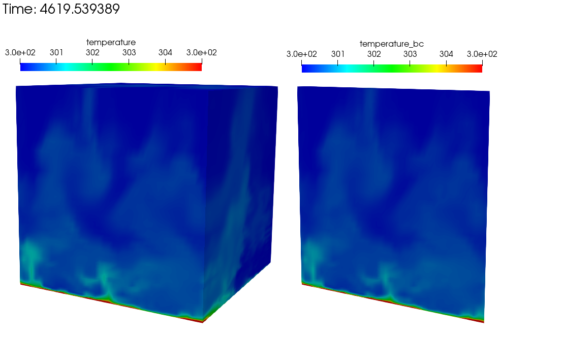
8.6 Subsequent simulation showing the full temperature domain (left) and on the precursor inflow temperature boundary condition field obtained from the perspective of the subsequent “external_field_provider” Realm (right).

9. Boussinesq Verification

9.1. Unit tests

Unit-level verification was performed for the Boussinesq body force term (2.9) with a nodal source. Proper volume integration with different element topologies is also tested (the “volume integration” tests in the MasterElement and HOMasterElement test cases).

9.2. Stratified MMS

A convergence study using the method of manufactured solutions (MMS) was also performed to assess the integration of the source term into the governing equations. An initial condition of a Taylor-Green vortex for velocity, a zero- gradient pressure field, and a linear enthalpy profile in the z-direction are imposed.

(9.43)$$\begin{array}{rl}u& =-\frac{1}{2}cos(2\pi x)sin(2\pi y)sin(2\pi z)\\ v& =sin(2\pi x)cos(2\pi y)sin(2\pi z)\\ w& =-\frac{1}{2}sin(2\pi x)sin(2\pi y)cos(2\pi z)\\ p& =0\\ h& =z.\end{array}$$

The simulation is run on a three-dimensional domain ranging from -1/2:+1/2 with reference density, reference temperature and the thermal expansion coefficient to equal to 1, 300, and 1, respectively. $\beta$ is much larger than typical ($1/T_{\mathrm{r}\mathrm{e}\mathrm{f}}$) so that the buoyancy term is a significant term in the MMS in this configuration.

The Boussinesq buoyancy model uses a gravity vector of magnitude of ten in the z-direction opposing the enthalpy gradient, $g_i=(0,0,-10{)}^T$. The temperature for this test ranges between 250K and 350K. The test case was run with a regular hexahedral mesh, using the edge-based vertex centered finite volume scheme. Each case was run with a fixed maximum Courant number of 0.8 relative to the specified solution.

9.1 Error in x-component of velocity

h	$L_{\mathrm{\infty }}$	L1	L2	Order
1/32	8.91e-3	1.12e-3	1.77e-3	NA
1/64	2.03e-3	3.04e-4	4.27e-4	2.05
1/128	4.65e-4	7.64e-5	1.05e-4	2.03

9.2 Error in y-component of velocity

h	$L_{\mathrm{\infty }}$	L1	L2	Order
1/32	1.78e-2	2.31e-3	3.47e-3	NA
1/64	4.18e-3	5.92e-4	8.23e-4	2.06
1/128	9.70e-4	1.50e-4	2.02e-4	2.03

9.3 Error in z-component of velocity

h	$L_{\mathrm{\infty }}$	L1	L2	Order
1/32	8.68e-2	1.17e-3	1.73e-3	NA
1/64	2.00e-3	2.99e-4	4.22e-4	2.04
1/128	4.64e-4	7.63e-5	1.05e-4	2.00

9.4 Error in temperature

h	$L_{\mathrm{\infty }}$	L1	L2	Order
1/32	1.09e-2	1.46e-3	2.10e-3	NA
1/64	2.06e-3	3.13e-4	4.19e-4	2.32
1/128	4.18e-4	7.54e-5	1.00e-4	2.06

This test is added to Nalu-Wind’s nightly test suite, testing that the convergence rate between the 1/32 and 1/64 element sizes is second order.

10. 3D Hybrid 1x2x10 Duct: Specified Pressure Drop

In this section, a specified pressure drop in a simple 1x2x10 configuration is run with a variety of homogeneous blocks of the following topology: hexahedral, tetrahedral, wedge, and thexahedral. This analytical solution is given by an infinite series and is coded as the “1x2x10” user function. The simulation is run with an outer wall boundary condition with two open boundary conditions. The specified pressure drop is 0.016 over the 10 cm duct. The density and viscosity are 1.0e-3 and 1.0e-4, respectively. The siumulation study is run a fixed Courant numbers with a mesh spacing ranging from 0.2 to 0.025. Figure 10.10 provides the standard velocity profile for the structured hexahedral and unstructured tetrahedral element type.

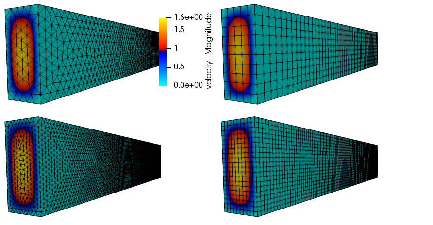
10.10 Streamwise velocity profile for specified pressure drop flow; tetrahedral and hexahedral topology.

The simulation study employed a variety of elemental topologies of uniform mesh spacing as noted above. Figure 10.11 outlines the convergence in the $L_2$ norm using the low-order elemental CVFEM implementation using the recently changed tetrahedral and wedge element quadrature rules. Second-order accuracy is noted. Interestingly, the hexahedral and wedge topology provided nearly the same accuracy. Also, the tetrahedral accuracy was approximately four tiomes greater. Finally, the Thexahedral topology proved to be second-order, however, provided very poor accuracy results.

10.11 $L_2$ error for the CVFEM scheme on a variety of element types.

11. 3D Hybrid 1x1x1 Cube: Laplace

The standard Laplace operator is evalued on the full set of low-order hybrid topologies (not inlcuding the pyramid). In this example, the temperature field is again,

(11.1)$$T=\frac{\lambda }{4}(cos(2a\pi x)+cos(2a\pi y)+cos(2a\pi z)).$$

Figure 11.1 represents the MMS field for temperature on a variety of mesh topologies. The thexahedral mesh is obtained from the standard uniform spacing tetrahedral mesh (not shown). The tetrahedral mesh shown is a tet-based conversion of the standard structured hexahedral mesh. This approach ensures that the number of nodes between the hexahedral and tetrahedral mesh are the same.

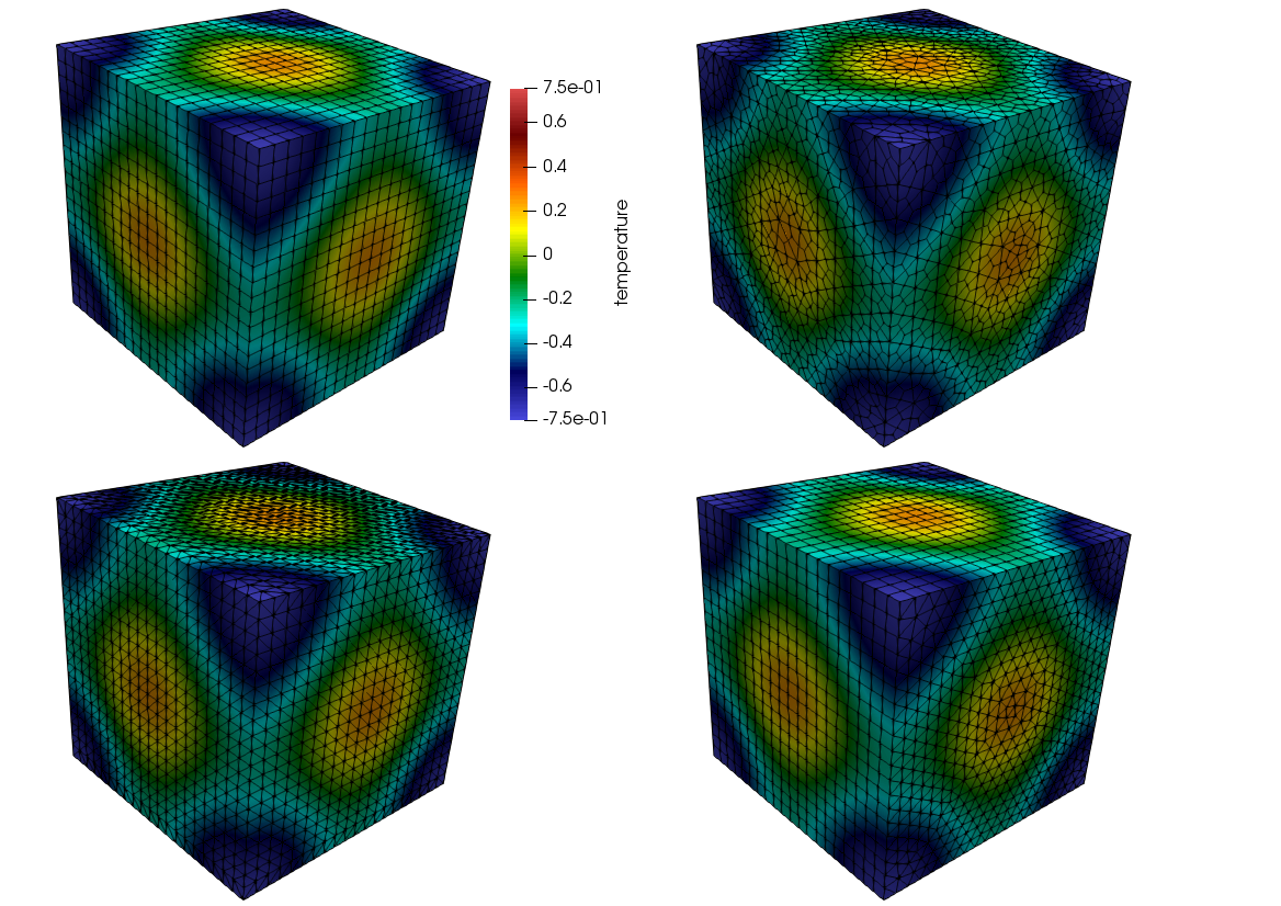
11.1 Temperature shadings for hexahedral, thexahedral, wedge, and tetrahedral topologies (clockwise from the upper left).

Figure 11.2 provides the $L_2$ norms, all of which are showing second-order accuracy. In Figure 11.3, the $L_o$ error is shown. As indicated from the convergence plot, slight degradation in order-of-accuracy is noted for the thexahedral topology.

11.2 $L_2$ norms for the full set of hybrid Laplace MMS study.

11.3 $L_o$ norms for the full set of hybrid Laplace MMS study.

12. Fixed Wing Verification Problem

Introduction A basic verification of the actuator line theory can be done by considering a fixed, 2D wing in a uniform flow. Such a test can be done independently of the openFAST library and can be easily verified by a simple algebraic calculation.

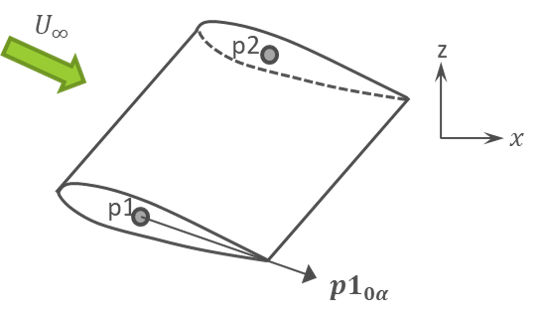
12.1 Schematic of the fixed wing airfoil problem.

An example of the fixed wing specification in the Nalu-Wind input file is shown below. The actuator type can be ActLineSimpleNGP for the NGP version and ActLineSimple for the non-NGP version (soon to be deprecated).

actuator:
  type: ActLineSimple
  search_method: stk_kdtree
  search_target_part: Unspecified-2-HEX

  n_simpleblades: 1
  debug_output: false
  n_turbines_glob: 0
  Blade0:
    num_force_pts_blade: 20
    epsilon: [3.0, 3.0, 3.0]
    p1: [-25, -4, 0]
    p2: [-25,  4, 0]
    p1_zero_alpha_dir: [1, 0, 0]
    chord_table: [1.0]
    twist_table: [0.0]
    aoa_table: [-180, 0, 180]
    cl_table:  [-19.739208802178716, 0, 19.739208802178716]
    cd_table:  [0]

The fixed wing is defined between points ${\mathbf{p}}_{\mathbf{1}}$ and ${\mathbf{p}}_{\mathbf{2}}$ given the chord length and blade twist defined in chord_table and twist_table. The direction ${\mathbf{p}\mathbf{1}}_{0\alpha }$ corresponding to the zero degree angle of attack is given in p1_zero_alpha_dir. The lift coefficients $C_L$ and drag coefficients $C_D$ are tabulated in the cl_table and cd_table parameters, respectively, as functions of the angle of attack $\alpha$ in aoa_table.

The lift $L$ and drag $D$ on the fixed wing can be calculated by infinite 2D airfoil theory using the formulas:

(12.3)$$L=\frac{1}{2}\rho U^2{C}_L(\alpha )S$$

(12.4)$$D=\frac{1}{2}\rho U^2{C}_D(\alpha )S$$

In equations (12.3) and (12.4), the area of the airfoil is given by $S$, the density is given by $\rho$, and the wind speed is given by $U$.

For the verification problem, a simple 2D, extruded blade is used with span $l=\text{8m}$ and chord $c=\text{1m}$, giving an area $S=8{\text{m}}^2$. An isotropic force spreading value of $\epsilon =3$ is used, along with 20 blade stations. The wind conditions are given by $\rho =1.0{\text{ kg/m}}^3$ and $U=2\text{ m/s}$.

The aerodynamic properties of the fixed wing are given by the linear lift coefficient

(12.5)$$C_L=2\pi \alpha$$

and zero drag

(12.6)$$C_D=0.$$

A comparison of total lift force calculated Nalu-Wind against the 2D airfoil theory is shown in Figure 12.2. As expected, the total lift force varies linearly with the angle of attack, and the agreement between theory and Nalu-Wind is good. Differences between the two methods were seen to be less than 0.1% over the range $0\le \alpha \le 5$ degrees.

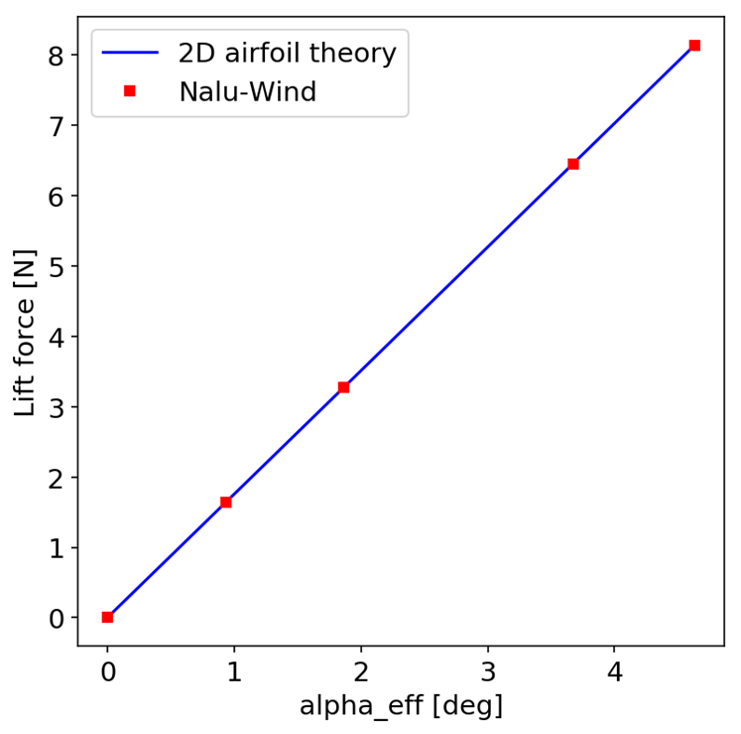
12.2 Comparison of the total lift force from Nalu-Wind and from 2D airfoil theory.

13. Actuator line simulations coupled to OpenFAST

We test the implementation of the actuator line algorithm in Nalu-Wind coupled to OpenFAST by performing a simulation of a flow past an elliptic wing at a constant angle of attack. We compare the solution from the coupled simulation to that using lifting line theory [KP02].

The elliptic wing is modeled using OpenFAST, a aero-hydro-servo-elastic tool to model wind turbines developed by the National Renewable Energy Laboratory (NREL). A static wind turbine model was created in OpenFAST with just one elliptic wing and all other systems including structural deformation, controls, etc. are turned off. The elliptic wing simulated in this work is an infinitesimally thin wing with a maximum chord ($c_0$) of $1m$ and an aspect ratio ($b/c_0$) of 10.0. The lift-curve slope ($d{C}_l/d\alpha$) of all airfoil sections on the wing is assumed to be $2\pi$ with no pressure or viscous drag. Using lifting line theory [KP02], the loads on the elliptic wing are

$$\begin{array}{rlr}\text{Area }S& =& \pi \frac{c_0}{2}\frac{b}{2},\\ \text{Maximum circulation }{\mathrm{\Gamma }}_{\max }& =& \frac{2b{U}_{\mathrm{\infty }}(\alpha -{\alpha }_{L0})}{1+4b/2\pi c_0},\\ \text{Lift coefficient }{C}_L& \equiv & \frac{L}{0.5\rho U_{\mathrm{\infty }}^{2}S}=\frac{\pi }{2}\frac{b}{S}\frac{{\mathrm{\Gamma }}_{\max }}{U_{\mathrm{\infty }}},\\ \text{Lift coefficient }{C}_D& \equiv & \frac{D}{0.5\rho U_{\mathrm{\infty }}^{2}S}=\frac{\pi }{4S}\frac{{\mathrm{\Gamma }}_{\max }^2}{U_{\mathrm{\infty }}^2},\\ \text{Constant induced downwash }{w}_i& =& \frac{{\mathrm{\Gamma }}_{\max }}{2b}.\end{array}$$

(13.1)$$\begin{array}{rl}\text{Span }b=& 10m\\ \text{Max chord }{c}_0=& 1.0m\\ \text{Angle of attack }\alpha =& 7^{\circ }\\ U_{\mathrm{\infty }}=& 10.0m/s\\ Reynolds\text{ number based on chord }=& 0.66M\\ \text{Number of actuator points across span }=& 50\end{array}$$

The flow past the elliptic wing is simulated in a domain of size $4b\times 3b\times 3b$. Some parameters of the simulation are described in equation (13.1). As described in the section Wind Turbine Modeling, the actuator line algorithm solves the momentum equation with a body force term spread to the nodes where $ϵ$ is the spreading width. It is necessary to maintain a constant $ϵ$ to observe convergence of the solution with grid refinement. However, we do expect the solution from the actuator line algorithm to be closer to that from lifting line theory with reducing $ϵ$. Hence, we perform five numerical simulations with grid resolutions as shown in table shown below. Simulations a,b,c use $ϵ=1m$ and d,e use $ϵ=0.5m$. We expect to see grid convergence with simulations a,b,c while we expect simulations d,e to predict a solution closer to the lifting line solution compared to simulations a,b,c.

Case	$\mathrm{\Delta }x/c_0$	$\mathrm{\Delta }t$	$ϵ/\mathrm{\Delta }$
a	0.125	0.00125	8.0
b	0.25	0.0025	4.0
c	0.5	0.005	2.0
d	0.125	0.00125	4.0
e	0.25	0.0025	2.0

The data shown in 13.1 - 13.5 are computed purely using output from OpenFAST. Unfortunately OpenFAST can only output data at a maximum of 9 stations along the blade. For this specific work, I had designed the aerodynamics module (AeroDyn) inside OpenFAST to use 18 stations to compute the forces along the blade. However, the mesh mapping algorithm in OpenFAST is used to interpolate the forces per unit length along the blade into discrete point forces at 50 actuator points along the blade as described in equation (13.1).

13.1-13.2 shows the comparsion of lift and drag coefficient predicted by the actuator line simulations to the solution from lifting line theory. Simulations d and e are closer to the lifting line solution compared to a,b,c because of the smaller $ϵ$. Simulations a,b,c show grid convergence since they use the same $ϵ$. 13.3-13.4 show similar results through the span wise distribution of the lift and drag per unit length along the blade. 13.5 shows the comparison of the predicted angle of attack on the blade to the constant angle attack predicted by the lifting line theory. As expected, the agreement with the lifting line theory is much better near the mid-span region compared to the wing tips.

13.1 Comparison of lift coefficient $C_L$ for an elliptic wing simulated using actuator line algorithm to solution using lifting line theory.

13.2 Comparison of drag coefficient $C_D$ for an elliptic wing simulated using actuator line algorithm to solution using lifting line theory.

13.3 Comparison of lift coefficient $C_L$ for an elliptic wing simulated using actuator line algorithm to solution using lifting line theory. Results are only shown at 9 different stations along the blade that are output from OpenFAST.

13.4 Comparison of drag coefficient $C_D$ for an elliptic wing simulated using actuator line algorithm to solution using lifting line theory. Results are only shown at 9 different stations along the blade that are output from OpenFAST.

13.5 Comparison of angle of attack distribution on an elliptic wing simulated using actuator line algorithm to solution using lifting line theory. Results are only shown at 9 different stations along the blade that are output from OpenFAST.

---

14. Open Boundary Condition With Outflow Thermal Stratification

In situations with significant thermal stratification at the outflow of the domain, the standard open boundary condition alone is not adequate because it requires the specification of motion pressure at the boundary, and this is not known a priori. Two solutions to this problem are: 1) to use the global mass flow rate correction option, or 2) to use the standard open boundary condition in which the buoyancy term uses a local time-averaged reference value, rather than a single reference value.

We test these open boundary condition options on a simplified stratified flow through a channel with slip walls. The flow entering the domain is non-turbulent and uniformly 8 m/s. The temperature linearly varies from 300 K to 310 K from the bottom to top of the channel with compatible, opposite-sign heat flux on the two walls to maintain this profile. The Boussinesq buoyancy option is used, and the density is set constant to 1.17804 kg/m ${}^3$. This density is compatible with the reference pressure of 101325 Pa and a reference temperature of 300 K. The viscosity is set to 1.0e-5 Pa-s. The flow should keep its inflow velocity and temperature profiles throughout the length of the domain.

The domain is 3000 m long, 1000 m tall, and 20 m wide with 300 x 100 x 2 elements. The upper and lower boundaries are symmetry with the specified normal gradient of temperature option used such that the gradient matches the initial temperature profile with its gradient of 0.01 K/m. Flow enters from the left and exits on the right. The remaining boundaries are periodic.

We test the problem on three configurations: 1) using the standard open boundary condition, 2) using the global-mass-flow-rate-correction option, and 3) using the standard open boundary condition with a local moving-time-averaged reference temperature in the Boussinesq buoyancy term.

Figure 14.1 shows the across-channel profile of outflow streamwise velocity. It is clear that in configuration 1, the velocity is significantly distorted from the correct solution. Configurations 2 and 3 remedy the problem. However, if we reduce the range of the x-axis, as shown in Figure 14.2, we see that configuration 3, the use of the standard open boundary condition with a local moving-time-averaged Boussinesq reference temperature, provides a superior solution in this case. In Figure, 14.3, we also see that configuration 1 significantly distorts the temperature from the correct solution.

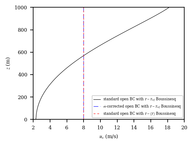
14.1 Outflow velocity profiles for the thermally stratified slip-channel flow.

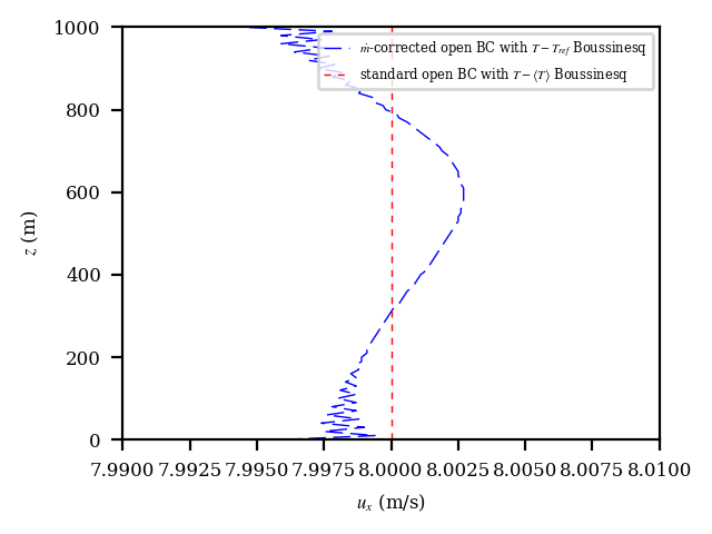
14.2 Outflow velocity profiles for the thermally stratified slip-channel flow considering only the case with the global mass-flow-rate correction and the standard open boundary with the local moving-time-averaged Boussinesq reference value.

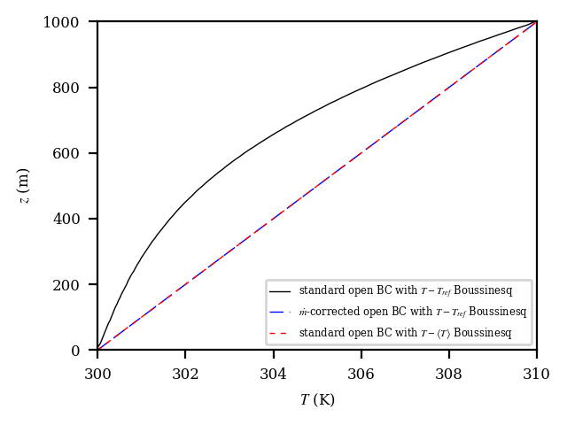
14.3 Outflow temperature profiles for the thermally stratified slip-channel flow.

We also verify that the global mass-flow-rate correction of configuration 2 is correcting the outflow mass flow rate properly. The output from Nalu-Wind showing the correction is correct and is shown as follows:

Mass Balance Review:
Density accumulation: 0
Integrated inflow:    -188486.0356751138
Integrated open:      188486.035672821
Total mass closure:   -2.29277e-06
A mass correction of: -2.86596e-09 occurred on: 800 boundary integration points:
Post-corrected integrated open: 188486.0356751139

15. Specified Normal Temperature Gradient Boundary Condition

The motivation for adding the ability to specify the boundary-normal temperature gradient is atmospheric boundary layer simulation in which the upper portion of the domain often contains a stably stratified layer with a temperature gradient that extends all the way to the upper boundary. The desire is for the simulation to maintain that gradient throughout the simulation duration.

Our test case is a laminar infinite channel with slip walls. In this case, the flow velocity is zero so the problem is simply a heat conduction through fluid. The density is fixed as constant, and there are no source terms including buoyancy.

This problem has an the analytical solution for the temperature profile across the channel:

(15.14)$$T(t,z)=T(t_0,z_0)+\frac{-g_H-g_0}{H}{\kappa }_{eff}(t-t_0)+g_0(z-z_0)+\frac{-g_H-g_0}{2H}(z-z_0{)}^2,$$

where $t_0$ is the initial time; $z_0$ is the height of the lower channel wall; $H$ is the channel height; $g_0$ and $g_H$ are the wall-normal gradients of temperature at the lower and upper walls, respectively; ${\kappa }_{eff}$ is the effective thermal diffusivity; and $z$ is the distance in the cross-channel direction. The sign of the temperature gradients assumes that boundary normal points inward from the boundary. For this solution to hold, the initial solution must be that of (15.14) with $t=t_0$.

For all test cases, we use a domain that is 10 m x 10 m in the periodic (infinite) directions, and 100 m in the cross-channel (z) direction. We specify a constant density of 1 kg/m ${}^3$, zero velocity, no buoyancy source term, a viscosity of 1 Pa-s, and a laminar Prandtl number of 1. No turbulence model is used. The value of $T(t_0,z_0)$ is 300 K.

15.1. Simple Linear Temperature Profile: Equal and Opposite Specified Temperature Gradients

A simple verification test that is representative of a stable atmospheric capping inversion is to compute the simple thermal channel with equal and opposite specified temperature gradients on each wall. By setting $g_H=-g_0$ in Equation (15.14), we are left with

(15.15)$$T(z)=T(z_0)+g_0(z-z_0).$$

In other words, if we set the initial temperature profile to that of (15.15), with $g_H=-g_0$, the profile should remain fixed for all time. In this case, we set $g_0=0.01$ K/m and $g_H=-0.01$ K/m.

We use a mesh that 2 elements wide in the periodic directions and 20 elements across the channel. We simulate a long time period of 25,000 s. Figure 15.3 shows that the computed and analytical solutions agree.

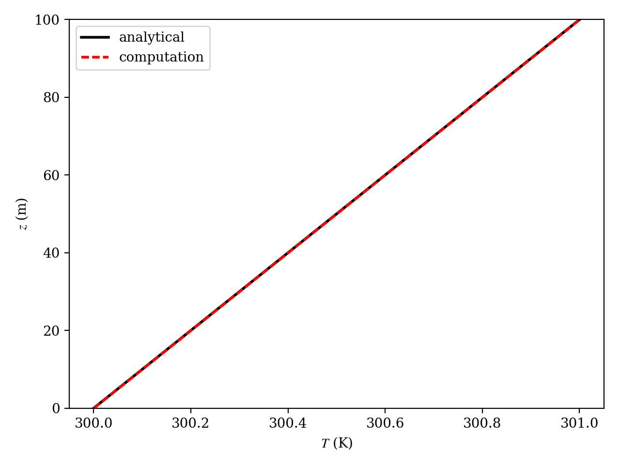
15.3 The analytical (black solid) and computed (red dashed) temperature profile from the case with $g_H=-g_0$ at $t=$ 25,000 s.

15.2. Parabolic Temperature Profile: Equal Specified Temperature Gradients

Next, we verify the specified normal temperature gradient boundary condition option by computing the simple thermal channel with equal specified temperature gradients, which yields the full time-dependent solution of Equation (15.14). Here, we set $g_0=g_H=0.01$ K/m.

We use meshes that are 2 elements wide in the periodic directions and 20, 40, and 80 elements across the channel. We simulate a long time period of 25,000 s. Figure 15.4 shows that the computed and analytical solutions agree. There is no apparent overall solution degradation on the coarser meshes.

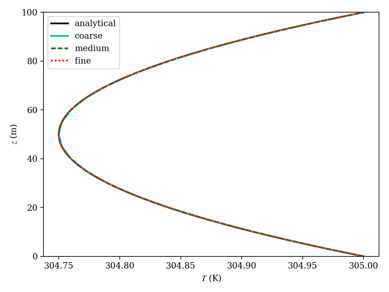
15.4 The analytical (black solid) and computed (colored) temperature profile from the case with $g_H=g_0$ at $t=$ 25,000 s.