Section: Sampling

This section controls data-sampling actions supported within AMR-Wind. The input parameters below use the label sampling as an example, as if this was provided to incflo.post_processing in the input file. For more information on specifying when sampled data is output to a file, see the post-processing inputs

sampling.output_format

type: String, optional, default = “native”

Specify the format of the data outputs. Currently the code supports the following formats

native

AMReX particle binary format. This is the preferred output format for performance.

ascii

AMReX particle ASCII format. Note, this can have significant impact on performance and must be used for debugging only.

netcdf

This requires linking to the netcdf library. If netcdf is linked to AMR-Wind and output format is not specified then netcdf is chosen by default.

sampling.labels

type: List of one or more names

Labels indicate the names of the different types of samplers (e.g., line, plane, probes) that are used to sample data from the flow field.

For example, if the user uses

Example:

sampling.labels = line1 lidar1 plane1 probe1

Then the code expects to read sampling.line1, sampling.plane1, sampling.probe1 sections to determine the specific sampling probe information.

sampling.fields

type: List of one or more strings

List of CFD simulation fields to sample and output

sampling.int_fields

type: List of one or more strings

List of CFD simulation int fields to sample and output (e.g. mask_cell)

sampling.derived_fields

type: List of one or more strings

List of CFD simulation derived fields to sample and output (e.g. mag_vorticity)

AMReX particle binary format

The native format can be read by ParaView or using Python scripts. We provide an example in the source code and the post processing documentation. A typical data frame might look like:

       uid  set_id  probe_id          xco     yco    zco  velocityx  velocityy  velocityz
  0      0       0         0   200.000000   200.0  200.0   6.129077   5.143022        0.0
  1      1       0         1   244.444444   200.0  200.0   6.129077   5.144596        0.0
 ..    ...     ...       ...          ...     ...    ...        ...        ...        ...
595    595       1       195   555.555556  1000.0  999.0   6.128356   5.142301        0.0
596    596       1       196   666.666667  1000.0  999.0   6.128356   5.142301        0.0

where uid is the global probe id, set_id is the label id (e.g., plane_sampling.labels = plane1 plane2, numbered as the user input order), probe_id is the local probe id to this label, *co are the coordinates of the probe, and the other columns are the user requested sampled fields. The same labels are seen by other visualization tools such as ParaView. The directory also contains a sampling_info.yaml YAML file where additional information (e.g., time) is stored. This file is automatically parsed by the provided particle reader tool and the information is stored in a dictionary that is a member variable of the class.

Sampling along a line

The LineSampler allows the user to sample the flow-field along a line defined by start and end coordinates with num_points equidistant nodes.

Example:

sampling.line1.type       = LineSampler
sampling.line1.num_points = 21
sampling.line1.start      = 250.0 250.0 10.0
sampling.line1.end        = 250.0 250.0 210.0

Sampling along a line moving in time (virtual lidar)

The LidarSampler allows the user to sample the flow-field along a line defined by origin and spanning to length with num_points equidistant nodes. Location of the line is given by the time histories azimuth_table and elevation_table. Angles are given in degrees with 0 azimuth and 0 elevation being the x direction. Lidar measurements may also be collected at a constant location by specifying only one entry to the tables.

Example:

sampling.lidar1.type            = LidarSampler
sampling.lidar1.num_points      = 21
sampling.lidar1.origin          = 250.0 250.0 10.0
sampling.lidar1.length          = 500.0
sampling.lidar1.time_table      = 0 10.0
sampling.lidar1.azimuth_table   = 0 90.0
sampling.lidar1.elevation_table = 0 45.0

Sampling on one or more planes

The PlaneSampler samples the flow-field on two-dimensional planes defined by two axes: axis1 and axis2 with the bottom corner located at origin and is divided into equally spaced nodes defined by the two entries in num_points vector. Multiple planes parallel to the reference planes can be sampled by specifying the offset_vector vector along which the planes are offset for as many planes as there are entries in the offset array.

Example:

sampling.plane1.type          = PlaneSampler
sampling.plane1.axis1         = 1.0 0.0 0.0
sampling.plane1.axis2         = 0.0 0.0 1.0
sampling.plane1.origin        = 0.0 0.0 0.0
sampling.plane1.num_points    = 10 10
sampling.plane1.offset_vector = 1.0 0.0 0.0
sampling.plane1.offsets       = 0.0 2.0 3.0

Illustration of this example:

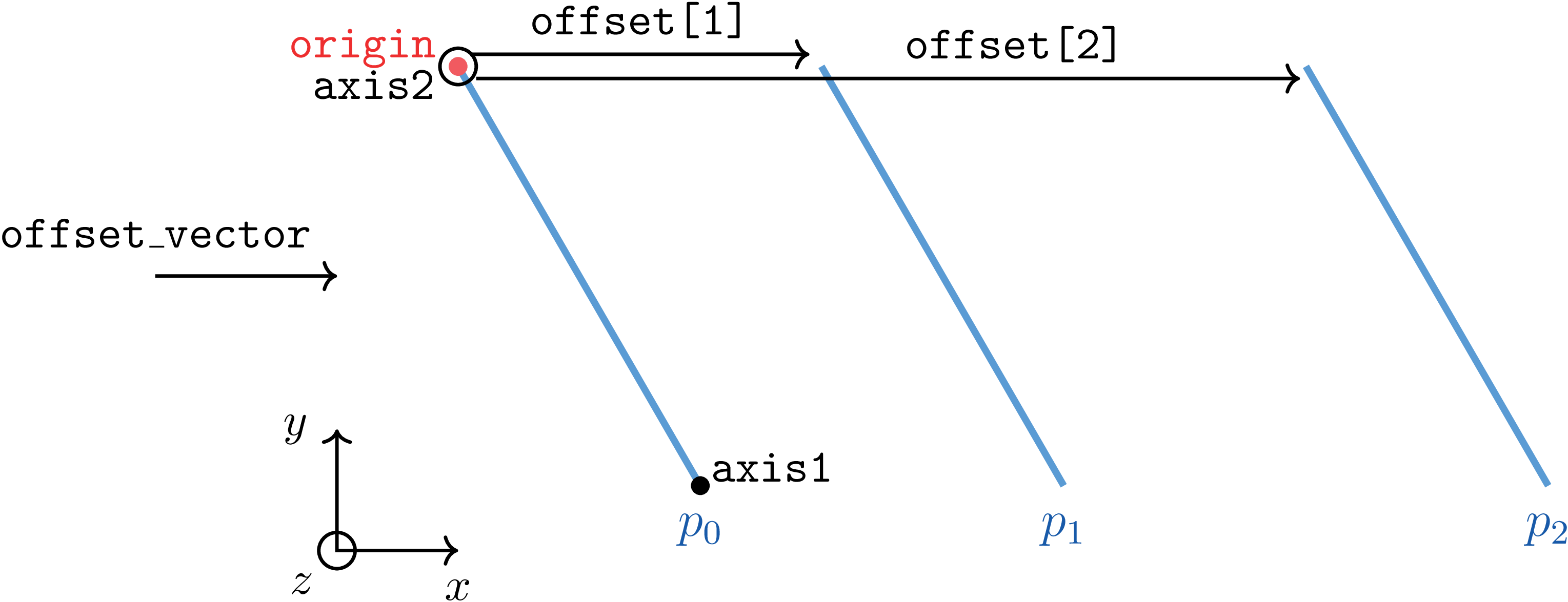
1 Example of sampling on planes.

Sampling at arbitrary locations

The ProbeSampler allows the user to sample the flow field at arbitrary locations read from a text file (default: probe_locations.txt).

Example:

sampling.probe1.type = ProbeSampler
sampling.probe1.probe_location_file = "probe_locations.txt"

The first line of the file contains the total number of probes for this set. This is followed by the coordinates (three real numbers), one line per probe. This type of sampler also supports the offset_vector and offsets options implemented with the plane sampler, shown above. For the probe sampler, these options apply offsets to the positions of all the points provided in the probe location file.

Sampling on a volume

The VolumeSampler samples a 3D volume that starts at lo and extends to hi. The resolution in all directions is specified by num_points.

Example:

sampling.volume1.type        = VolumeSampler
sampling.volume1.hi        = 3.0 1.0 0.5
sampling.volume1.lo      = 0.0 0.0 -0.5
sampling.volume1.num_points  = 30 10 10

Sampling on the air-water interface

The FreeSurfaceSampler samples on the air-water interface, and it requires the vof (volume-of-fluid) field to be present in order to function. The sample locations are specified using a grid that starts at plane_start and extends to plane_end. The resolution in each direction is specified by plane_num_points. The coordinates of the sampling locations are determined by the location of the air-water interface in the search direction, specified by search_direction, and the other coordinates are determined by the plane_ parameters. The default search direction parameter is 2, indicating the samplers will search for the interface along the z-direction. Due to this design, it is best to specify a plane that is normal to the intended search direction.

Another optional parameter is num_instances, which is available for cases where the interface location is multi-valued along the search direction, such as during wave breaking. This parameter defaults to 1, and the sampler will automatically select the highest position along the search direction when the interface location is multi-valued.

The free surface location is calculated with a geometric approach using the reconstruction of the interface in a computational cell. However, within the numerical beach of a wave simulation, the volume fraction distribution can become noisy, and the geometric approach produce noisy results. To avoid this, there is an option to use a linear interpolation approach instead within the beach, which helps to reduce the noise. This can be turned on using the argument linear_interp_extent_from_xhi, which specifies the extent from the upper domain boundary (in x) where linear interpolation should be used instead of the standard geometric approach. This input parameter should be set to the length of the numerical beach.

Example:

sampling.fs1.type             = FreeSurfaceSampler
sampling.fs1.plane_start      = 4.0 -1.0 0.0
sampling.fs1.plane_end        = 0.0 1.0  0.0
sampling.fs1.plane_num_points = 20 10